Gauss and the Fast Fourier Transform
The Fast Fourier Transform (FFT) is a modern algorithm to compute the Fourier coefficients of a finite sequence. Fourier will forever be known by his assertion in 1807 that any function could be expressed as a linear combination of sines and cosines, its Fourier series. "Any" was a little ambitious, counter-examples coming to the fore in due time. A fair amount of mathematics from that time to this has been devoted to refining Fourier's insight and studying trigonometric series, a subject that led Georg Cantor to founding set theory. Piecewise smoothness is sufficient for pointwise convergence on \( [-\pi, \pi] \):
\[ f(x) = {a_0 \over 2} + \sum_{j=1}^\infty \left( a_j \cos jx + b_j \sin jx \right), \]
where the Fourier coefficients are:
\[ a_m = {1 \over \pi} \int_{-\pi}^\pi f(x) \cos mx \,dx, \hspace{20 pt} b_m = {1 \over \pi} \int_{-\pi}^\pi f(x) \sin mx \,dx \hspace{20 pt} (m = 0, 1, 2, ...). \]
The finite version, known as the Discrete Fourier Transform (DFT), arises where the function \( f \) is known only at a sequence of sampled points. Then calculating the Fourier coefficients is a finite process and the FFT is a fast way to do it.
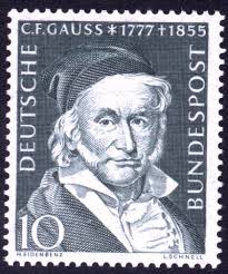
James Cooley of IBM and John Tukey of Princeton published the FFT algorithm in 1965, Tukey reportedly hatching the idea as a way of detecting nuclear-weapon tests in the Soviet Union (see the Wikipedia writeup and the original paper[1] - a little over four pages!). I almost wrote "discovered" the FFT, but the interesting thing is that the algorithm has a long pedigree going back to Gauss. A key source is the inimitable Herman Goldstine[2], who retraces Gauss in detail (§ 4.12). The work in question is Theoria Interpolationis Methodo Nova Tractata[3], written of course in Latin (The Theory of Interpolation Treated by a New Method) and first published in 1866 after being found among Gauss's papers after death. There is good evidence for a composition date of 1805, predating even Fourier - Gauss was 28 years old at the time (see Goldstine's footnote on page 253, noting that Gauss refers to "pro novo planeta Iunone", suggesting that the asteroid Juno had been recently discovered - it was discovered in 1804).
Recapitulating Gauss
Gauss has a long and difficult (for me), but intelligible, account of trigonometric interpolation, then says in §28, let's apply all that to the position of the recently discovered asteroid Pallas as found in Baron von Zach's tables (Gauss, pp 308-9, Goldstine, pp 251-2). "Trigonometric interpolation" means finding a function \( f \) as a sum of trigonometric functions passing through a sequence of N data points \( (x_n, y_n) \), so that \( y_n = f(x_n) \), where:
\[ \begin{equation}{f(x) = {1 \over 2} a_0 + \sum_{j=1}^{N/2-1} \left( a_j \cos jx + b_j \sin jx \right) + {1 \over 2} a_{N/2} \cos ({N \over 2} x).} \tag{1} \end{equation} \]
This formula is from Dahlquist and Björck[4], p 488, and assumes that the \( x_n \) are evenly spaced, that \( x_0 = 0 \), and that N is even (a slightly different formula obtains if N is odd). Note the similarity to the Fourier coefficients in the continuous case, the integrals towards the top of the page. They say the finite formulas are equivalent to:
\[ f(x) = \sum_{j=-N/2}^{N/2} c_j e^{ijx}, \]
where i = \( \sqrt{-1} \) and the \( c_j \) are complex numbers related to the \( a_j \) and \( b_j \) and with \( c_j = \overline{c_j} \) - the formulas for the coefficients are:
\[ a_j = {2 \over N} \sum_{k=0}^{N-1} f(x_k) \cos{j x_k}, \hspace{20 pt} b_j = {2 \over N} \sum_{k=0}^{N-1} f(x_k) \sin{j x_k}, \hspace{20 pt} c_j = {1 \over N} \sum_{k=0}^{N-1} f(x_k) e^{-i j x_k}. \]
Considering that \( e^{ijx} = \cos jx + i sin jx \), simple relations among these values can be derived for \( 0 \leq j < {{N/2}-1} \) :
\[ \begin{equation}{a_0 = 2 c_0, \hspace{16 pt} a_j = c_j + c_{-j} = 2 \Re(c_j), \hspace{16 pt} b_j = i({c_j - c_{-j}}) = -2 \Im(c_j), \hspace{16 pt} a_{N/2} = 2 c_{N/2}} \tag{2} \end{equation} \]
The sequence \( \{c_j \} \) constitutes the Inverse Discrete Fourier Transform (IDFT) of the sequence \( \{ y_n \} \) - the two sequences have the same number of elements and the IDFT takes \( \mathbb{C}^N \rightarrow \mathbb{C}^N \) in general, even though our input sequences here consist of real numbers. The DFT is almost identical, with \( e^{+i j x_k} \) used in the formula instead of \( e^{-i j x_k} \). Either way, these values are roots of unity spread evenly around the circle, so you are traversing the same values, just in a different direction, clockwise or counter-clockwise.
Gauss's data, the \( (x_n, y_n) \) he wants to interpolate and fit with sines and cosines, gives the declination of Pallas in minutes (y) as a function of the right ascension in degrees (x):
| x | y |
|---|---|
| 0 | 408 |
| 30 | 89 |
| 60 | -66 |
| 90 | 10 |
| 120 | 338 |
| 150 | 807 |
| 180 | 1238 |
| 210 | 1511 |
| 240 | 1583 |
| 270 | 1462 |
| 300 | 1183 |
| 330 | 804 |
Table 1
Graph 1
That's a twelve point interpolation, but Gauss says let's do the interpolation for every third pair first, the red ones above with N = 4 and (using radians) \( (x_n, y_n) = \{(0,408), (\pi/2, 10), (\pi, 1238), (3\pi/2, 1462)\} \). The graph on the right is the interpolating function, calculated as follows, using the formulas in (2):
\[ {{1 \over 2} a_0 = {1 \over 2} {2 \over 4} \sum_{k=0}^3 y_k \cos {(0 \cdot x_k)}} = {1 \over 4} ({y_0 + y_1 + y_2 + y_3}). \]
\[ {a_1 = {2 \over 4} \sum_{k=0}^3 y_k \cos {(1 \cdot x_k)}} = {1 \over 2} ({y_0 \cos 0+ y_1 \cos \pi/2+ y_2 \cos 3 \pi /2+ y_3 \cos 2 \pi}) = {{y_0 - y_2} \over 2}. \]
\[ {b_1 = {2 \over 4} \sum_{k=0}^3 y_k \sin {(1 \cdot x_k)}} = {1 \over 2} ({y_0 \sin 0+ y_1 \sin \pi/2+ y_2 \sin 3 \pi /2+ y_3 \sin 2 \pi}) = {{y_1 - y_3} \over 2}. \]
\[ {a_2 = {1 \over 2} {2 \over 4} \sum_{k=0}^3 y_k \cos {(2 \cdot x_k)}} = {1 \over 4} ({y_0 \cos 0+ y_1 \cos \pi+ y_2 \cos 2 \pi + y_3 \cos 3 \pi}) = {{y_0 - y_1 + y_2 - y_3} \over 4}. \]
Plugging in the y values leads to \( \{{a_0 / 2}, a_1, b_1, {a_2 / 2}\} = \{ 779.5, -415, -726, 43.4 \} \), so:
\[ \boxed{f(x) = 779.5 -415 \cos x -726 \sin x + 43.5 \cos {2 x}} \]
which agrees with Gauss (Goldstine, top of p 252). Plug the \( (x_n, y_n) \) into this equation to see that it does indeed interpolate the data - this is the graph shown above. The calculations can be teased out of Gauss, but it's hard slogging with his A, B, C, D instead of \( y_n \), Greek letters like \( \gamma \) and \( \delta' \) for the Fourier coefficients, and endless subcases - even the letter \( \pi \) serves as a variable. You come away with great appreciation for modern notation and enhanced respect for the master who didn't have it at his disposal.
The Remaining Tetrads
Next is another interpolation problem with the pairs immediately following the red ones in Table 1, where \( (x_n', y_n') = \{(\pi/6, 89), (2\pi/3, 338), (7\pi/6, 1511), (5\pi/3, 1183)\} \). This one is complicated by the fact that \( x_0 = \pi/6 \), and the Dahlquist formulas require that \( x_0 = 0 \). No problem - we assume \( x_0 = 0 \) as above and at the last step translate by \( \pi/6 \) using the addition formulas for sine() and cosine(). The formulas are straightforward, but a bit arduous with sixteen sine() and cosine() evaluations. Alpha Wolfram can be used with command lines like this for the second calculation of the four:
1/2{89,338,1511,1183}.Table[cos((m-1)pi/2),{m,4}]
Alpha Wolfram's Table enables vector building and the dot just before it is the dot product, so we have a sum of products, as desired. \( m \) increments by 1 starting at 1, by default, and stopping at 4, so the expression \( \cos((m-1)pi/2) \) advances through \( \{0, \pi/2, \pi, 3\pi/2\} \), as when manually calculated above. The result is -711, and after translating by \( \pi/6 \) there is a \( \sin(2x) \) component as well introduced when expanding \( \cos(2(x-\pi/6)) \):
\[ \begin{equation}{\boxed{g(x) = 780.25 - 404.494 \cos x - 721.396 \sin x + 9.875 \cos {2 x} + 17.104 \sin {2 x}}} \tag{3} \end{equation} \]
The third tetrad of values can be developed into a third function similarly. Here is the general function and table in Goldstine (bottom of page 251 and top of page 252) straight from Gauss, where the Greek letters are the coefficients of the sines and cosines of the three functions (notation following Gauss, where \( X' \) is not a derivative):
\[ \begin{equation}{\boxed{X' = \gamma + \gamma' \cos x + \delta' \sin x + \gamma'' \cos {2 x} + \delta'' \sin {2 x}}} \tag{4} \end{equation} \]
| Pro periodo | ubi y = 4x | \( \gamma \) | \( \gamma' \) | \( \ \delta' \) | \( \gamma'' \) | \( \ \delta'' \) |
|---|---|---|---|---|---|---|
| prima | 0 ° | +779.5 | -415.0 | -726.0 | +43.5 | 0 |
| secunda | 120 ° | +780.2 | -404.5 | -721.4 | +9.9 | +17.1 |
| tertia | 240 ° | 782.0 | -413.5 | -713.3 | +11.7 | -20.3 |
Table 2
Worked Example - Trigonometric Interpolation
Let's pause in the exegesis of Gauss for a moment to make sure the method is understood, taking up an example with N = 6 and showing how to streamline the calculation with Alpha Wolfram's ifft() command, which produces IDFTs. Let the points to interpolate be \( (x_n, y_n) = \{(0, 8), (\pi/3, 5), (2\pi/3, -28), (\pi, -14), (4\pi/3, -8), (5\pi/3, -2)\} \). We want to find the interpolating trigonometric polynomial, to find the coefficients \( a_j \) and \( b_j \) in:
\[ t(x) = a_0 + a_1 \cos x + b_1 \sin x + a_2 \cos {2 x} + b_2 \sin {2 x} + a_3 \cos {3 x}. \]
So execute an inverse fft in Alpha Wolfram to get the \( c_j \).
\[ \begin{align} {ifft\{8, 5, -28, -14, -8, -2\} = \\ \{-15.9217, 16.9423+4.59619 i, 4.28661-9.54594 i, \\ -6.94022, 4.28661+9.54594 i, 16.9423-4.59619 i\}.} \end{align} \]
Graph 2
We want to apply the formulas in (2) at this point to get the \( a_j \) and \( b_j \), but confusion reigns because implementations of the fft / ifft sometimes multiply or divide the fft results by \( N \) or \( \sqrt{N} \). Alpha Wolfram's ifft() multiplies the results by \( \sqrt{N} \), so we must divide their results by \( \sqrt{N} \) (\( \sqrt{6} \) in this case):
\[ a_0 = -15.9217 / \sqrt{6} = -6.5 = -6 \frac{1}{2} \]
\[ a_1 = 2 \cdot 16.9423 / \sqrt{6} = 13.8333 = 13 \frac{5}{6} \]
\[ b_1 = -2 \cdot 4.59619 / \sqrt{6} = -3.75277 \]
\[ a_2 = 2 \cdot 4.28661 / \sqrt{6} = 3.5 = 3 \frac{1}{2} \]
\[ b_2 = -2 \cdot (-9.54594) / \sqrt{6} = 7.79422 \]
\[ a_3 = -6.94022 / \sqrt{6} = -2.8333 = -2 \frac{5}{6} \]
so:
\[ t(x) = -6.5 + 13 \frac{5}{6} \cos x - 3.75277 \sin x + 3 \frac{1}{2} \cos {2 x} + 7.79422 \sin {2 x} - 2 \frac{5}{6} \cos {3 x}. \]
The graph shows \( t(x) \), the curve in blue going through the six original interpolation points. The other curve in gray is the same as \( t(x) \), except leaving off the final \( \cos 3x \) term, illustrating that most of the information is in the lower frequencies, the higher ones being necessary for exactness. Compare to Taylor series, where most of the approximation is carried by the lower or higher powers of \( x \) depending on whether you're close to 0 or not.
The Fast Fourier Transform - Divide and Conquer
But let's return to Gauss, we left off in the middle. Referring to Table 2, Gauss says let's derive trigonometric functions for the columns, taking the column of \( \gamma \)s as data to be itself interpolated, and the same for the other columns of coefficients. Taking the \( \gamma \)s, the points to interpolate are \( \{(0, 779.5), (2 \pi / 3, 780.2), (4 \pi /3, 782.0) \} \). Here we have N=3 rather than being even and the formulas and approach are almost the same as for the N=4 case worked out above. The main difference is that there is not a final cosine term:
\[ \gamma = a_0' + a_1' \cos x + a_2' \sin x, \]
where
\[ a_1' = {{2 \over 3} (779.5 \cos 0 + 780.2 \cos {2 \pi / 3} + 782.0 \cos {4 \pi / 3})} = -1.06667 \]
Graph 3
and similarly for the other two coefficients, so (rounding):
\[ \gamma = 780.6 - 1.1 \cos x - 1.0 \sin x. \]
Here's a key step - put \( 4 x \) instead of \( x \) in this formula, the 4 arising from there being 4 groups at the first step (N=4):
\[ \gamma = 780.6 - 1.1 \cos 4 x - 1.0 \sin 4 x. \]
Develop similar expansions for the other \( \gamma \)s and \( \delta \)s:
\[ \gamma' = -411.0 - 4.0 \cos 4 x + 5.2 \sin 4 x, \]
\[ \delta' = -720.2 - 5.8 \cos 4 x - 4.7 \sin 4 x, \]
\[ \gamma'' = 21.7 + 21.8 \cos 4 x - 1.1 \sin 4 x, \]
\[ \delta'' = -1.1 + 1.1 \cos 4 x + 21.6 \sin 4 x, \]
Then plug these expressions into (4) and simplify using the product-to-sum identities, like:
\[ {\cos 4 x \cdot \sin 2 x} = {1 \over2} {(\sin{(4 x + 2 x)} - \sin{(4 x - 2 x)})} = {1 \over2} {(\sin 6 x - \sin 2 x)} \]
The final expansion is:
\[ \begin{align}{X''(x) = {780.6 - 411.0 \cos x - 720.2 \sin x + 43.4 \cos 2x - 2.2 \sin 2x - 4.3 \cos 3x + 5.5 \sin 3x \\
- 1.1 \cos 4x - 1.0 \sin 4x + 0.3 \cos 5x - 0.3 \sin 5x + 0.1 \cos 6x},} \end{align} \]
and this composite method interpolates the 12 points in Table 1 and produces the same result as doing the 12-point interpolation without the two part breakdown.
To see this, just reprise the derivations at the original twelve interpolation points, thinking of the \( \gamma \)s and \( \delta \)s as functions of \( 4 x \), like this:
\[ X''(\pi / 6) = {\gamma(2 \pi / 3) + \gamma'(2 \pi / 3) \cos x + \delta'(2 \pi / 3) \sin x + \gamma''(2 \pi / 3) \cos {2 x} + \delta''(2 \pi / 3) \sin {2 x}} \]
Those \( \gamma \) and \( \delta \) "coefficients" are the ones in the secunda row in Table 2 or my \( g(x) \) in (3) above, which interpolated the second triad of interpolation points, including \( \pi / 6 \). And the coefficients are the same that a 12-point interpolation would produce, because there is only one expansion with the sines and cosines going up to \( \cos(6 x) \). That's evident because the original interpolation problem could have been posed as solving 12 equations for 12 unknowns (the \( a_i \) and \( b_i \), and always solvable too, because the coefficient matrix is of the Vandermonde type).
Graph 3 places the final interpolating curve \( X'' \) over the earlier incomplete interpolating curve \( f(x) \) in Graph 1, the later being for the four points in the prima tetrad, marked by red dots in both graphs. Graph 3 shows the other eight points as well - green for the secunda tetrad and blue for tertia. Graph 3 emphasizes how very close the final curve is to the one interpolating only the prima points, that will vary based on the data set. Most of the information is in the lower frequencies, the higher frequencies being fine-tuning adjustments.
Computational Complexity
At which point you might be thinking, what's the point of complicating a problem that was a whole lot easier to start with. The answer is computational efficiency. I mentioned the term divide and conquer with respect to Gauss's interpolation example. His solution breaks the original 12-point problem into three four-point problems at the first step, then five three-point problems at the second step, and finally stitches them together for the solution. An \( M \)-point problem takes \( M^2 \) multiplications (the trigonometric evaluations can be hard-coded), so here's how many calculations each approach takes:
| Number of calculations | |
|---|---|
| Original 12-point: | 12 x 12 = 144 |
| Gauss version: | 3 x 42 + 5 x 32 = 3 x 16 + 5 x 9 = 48 + 45 = 93 |
Table 3
That's a savings, but a modest one. The key concept though, is that if the original number of points is highly composite, each sub-problem can itself be decomposed into two still smaller sub-problems. And on and on down to 1, accumulating savings. More generally, let \( N = N_1 \cdot N_2 \) be the number of points in the original problem, where we will decompose into \( N_2 \) sets of \( N_1 \) points - in the example, \( N_1 = 4 \) (the tetrads) and \( N_2 = 3 \). The 5 in the bottom row of Table 3 can be taken as 4 (\( N_1 \)) in more general implementations, so the decomposition reduces to:
\[ {\text{Number of calculations in decomposed problem}} = {{N_1^2 N_2} + {N_2^2 N_1} = {{N_1 N_2} ({N_1 + N_2})} = {N ({N_1 + N_2})}} \]
Of course \( {N_1 + N_2} < {N_1 N_2} = N \) and therein lies the savings. We're ready to start thinking of a cascading descent, so let's analyse the interpolation problem at the bottom of that descent, when \( N = 1 \) and \( N = 2 \). For \( N = 1, y_0 \) is the only point, so the interpolating function is \( t(x) = y_0 \), the number of calculations is 0. For For \( N = 2 \), let the points be \( \{y_0, y_1\} \), which we want to interpolate with \( s(x) = a_0 + a_1 \cos x \). Putting:
\[ y_0 = s(0) = a_0 + a_1 \cos 0, \hspace{20 pt} y_1 = s(\pi) = a_0 + a_1 \cos \pi, \]
and solving two equations for two unknowns leads to the solution \( \{a_0 = {{y_0 + y_1} \over 2}, a_1 = {{-y_0 + y_1} \over 2}\} \), two divisions, and that is overdoing it, because dividing by two on a computer is not a division at all, but a shift that is faster than addition. So say the number of calculations is 2.
Starting with \( N = 2 M \)points, we'll break the problem into M interpolations of 2 points, followed by 2 interpolations of M points; in the notation above: \( N_1 = 2, N_2 = M \). So if \( k(m) \) is a measure of the number of calculations in a \( m \) point problem:
\[ k(2 M) = {M \cdot k(2) + 2 \cdot k(M)} = {2M + 2 k(M)}, \]
or, recasting with \( n = M / 2 \):
\[ k(n) = {n + 2 \cdot k(n / 2)}. \]
This is a recurrence, a staple of computer science theory, not to say mathematics generally (as in the Fibonacci numbers, for example). See Chapter 4 of the most excellent Introduction to Algorithms[5], by Cormen, Leiserson, and Rivest, for an accessible account of this subject. In the instant case, put \( n = 2^p \) and repeatedly reduce by 2:
\[ \hspace{-58 pt} k(n) = {n + 2 \cdot k(n / 2)} \]
\[ \hspace{12 pt} = {n + 2 \cdot ({n / 2 + 2 \cdot k(n / 4)})} \]
\[ \hspace{-30 pt} = {2 n + 4 \cdot k(n / 4)} \]
\[ \hspace{17 pt} = {2 n + 4 \cdot ({n / 4 + 2 \cdot k(n / 8)})} \]
\[ \hspace{-30 pt} = {3 n + 8 \cdot k(n / 8)} \]
\[ \hspace{-30 pt} \vdots \]
\[ \hspace{12 pt} = {p n + n \cdot k(1)} = n \cdot log_2 n \]
| \( p = log_2 n \) | \( n = 2^p \) | \( n^2 \) | \( n log_2 n \) | \( n / log_2 n \) |
|---|---|---|---|---|
| 0 | 1 | 1 | 0 | - |
| 1 | 2 | 4 | 2 | 2.0 |
| 2 | 4 | 16 | 8 | 2.0 |
| 3 | 8 | 64 | 24 | 2.7 |
| 4 | 16 | 256 | 64 | 4.0 |
| 5 | 32 | 1024 | 160 | 6.4 |
| 6 | 64 | 4096 | 384 | 10.7 |
| 7 | 128 | 16,384 | 896 | 18.3 |
| 8 | 256 | 65,536 | 2048 | 32.0 |
| 9 | 512 | 262,144 | 4608 | 56.9 |
Table 4
The very last step is because \( k(1) = 0 \) and \( p = log_2 n \) is synonymous with \( n = 2^p \); \( p = log_2 n \) is the number of steps in this descent.
Consider Table 4. The fourth column shows that we are on the mark taking \( k(n) = n log_2 n \), because \( n log_2 n \) satisfies the recurrence: 384 = k(64) = 64 + 2·k(32) = 64 + 2·160, for example, and a simple induction on p proves it in general. The \( n^2 \) column shows the computational demand of an original problem with \( n \) points, the \( n log_2 n \) column the requirement for the same size problem using the FFT approach. The latter grows more slowly with \( n \), a little more than doubling while \( n^2 \) quadruples at every step. The last column shows the ratio, so that by the time \( n = 512 \), the ratio is \( 512 / 9 = 56.9 \). What took an hour the old way now takes a minute; that is something.
The FFT As Technology
It's no accident that the FFT was revived and appreciated just at the moment when machine calculation was becoming increasingly widespread in scientific institutions. This outline from Dima Batenk takes up the long history of the FFT (not much on Gauss though) and is convincing that the world was ready for the FFT in the late 1950s. See in particular the sections on I. J. Good starting on page 28 - he was a pioneer of the rediscovery and his paper is one of two Cooley and Tukey cited in 1965.
Heideman, Johnson, and Burrus wrote a canonical paper on this subject, "Gauss and the History of the Fast Fourier Transform"[6], the starting point for which was Goldstine's footnote on page 249 about Gauss and the FFT:
This fascinating work of Gauss was neglected and was rediscovered by Cooley and Tukey in an important paper in 1965.
Heideman et al. note that Runge and König had published a doubling algorithm for the DFT in 1924 and that is the FFT, at least for powers of two, a common implementation to this day. They give a number of references to FFT-like algorithms before and after Runge and König. In 1967, Cooley himself and associates Peter Lewis and Peter Welch wrote "Historical Notes on the Fast Fourier Transform"[7], which starts with this compact and informative statement:
The Fast Fourier Transform (FFT) algorithm is a method for computing the finite Fourier transform of a series of N (complex) data points in approximately Nlog2N operations. The algorithm has a fascinating history. When it was described by Cooley and Tukey in 1965 it was regarded as new by many knowledgeable people who believed Fourier analysis to be a process requiring something proportional to N2 operations with a proportionality factor which could be reduced by using the symmetries of the trigonometric functions. Computer programs using the N2-operation methods were, in fact, using up hundreds of hours of machine time. However, in response to the Cooley-Tukey paper, Rudnick, of Scripps Institution of Oceanography, La Jolla, Calif., described his computer program which also takes a number of operations proportional to Nlog2N and is based on a method published by Danielson and Lanczos. It is interesting that the Danielson-Lanczos paper described the use of the method in X-ray scattering problems, an area where, for many years after 1942, the calculation of Fourier transforms presented a formidable bottleneck to researchers who were unaware of this efficient method.
Even before 1965, then, technologists were implementing the algorithm and they were doing so in the 1930s before the advent of digital computers. People needed their Fourier expansions and were most interested in efficient methods when it could take hours to calculate a single transform with paper and pencil, only to later discover an error at step 1. They fashioned mathematical techniques and passed along the lore in their disciplines.
Tide prediction is an instructive example, where ship masters need accurate information about low and high tides that can easily vary by seven meters at a port (London here). As early as the 1830s, British scientists diligently collected and charted daily data. A sinusoidal pattern as a function of time was obvious, but for decades these charts were sufficient predictors and were preferred by the Admiralty into the 20th century. Sophisticated automatic data collection devices were devised in the course of the 19th century. In the mean time scientists like Lord Kelvin and George H. Darwin (son of Charles) started to advance a "harmonic" theory of tides based on Newtonian / Laplacian dynamics (harmonic = Fourier). They spoke of "constituents" or sometimes "tides", meaning the frequencies used to represent the function for water height at a given place as a function of time, and these constituents represented physical factors like the motions of the sun and moon and the earth's rotation. There could be thirty constituents or more. Kelvin brought these two streams together with his amazing tide-predicting machine, an analog computer evaluating the trigonometric polynomials theory produced at thousands of points to build tide tables better than those coming from raw data; these machines were in active service through the 1970s.
Heideman et al. say that George Darwin and his associates developed efficient Fourier methods circa 1880 and British and American scientists, the latter at the US Coast and Geodetic Survey, continued this tradition into the mid 20th century. It's just a big interpolation problem at each port. You've got extensive data and the task is to find the Fourier expansion interpolating it. The tale is well told in David Cartwright's Tides: A Scientific History[8]. A lot of it has lost its point today, fascinating though it is as a case study. That some minor perturbation of the moon's orbit contributes to the cos(13x) component in tide calculations may be highly interesting to theoretical astronomers and oceanographers, but for prediction, just interpolate with the data available for every hour of the year - that's just a 365 x 24 = 8760 point FFT!
The FFT story illustrates the material and practical foundation of much of mathematics - astronomy, tide predicting, and X-ray scattering being mentioned in the foregoing. It's not completely surprising to see Gauss staking a claim at the beginning, great bridge that he was between theoretical astronomy and mathematics. Some mathematicians and practitioners knew about FFT-like algorithms over the years; it's just that mathematicians were not terribly interested - there wasn't all that much you could do with it as a practical matter anyway, so why press the point.
Modern digital computers changed everything; the old lore was revisited and the old papers dusted off, recast, and generalized. Entire branches of science turned obsolete almost over night as the once unthinkable became routine.
Mike Bertrand
April 5, 2014
^ 1. "An Algorithm for the Machine Calculation of Complex Fourier Series", by James W. Cooley and John W. Tukey, Mathematics of Computation, 19: 297–301 (April, 1965).
^ 2. A History of Numerical Analysis from the 16th through the 19th Century, by Herman H. Goldstine, Springer-Verlag (1977), ISBN 0-387-90277-5.
^ 3. "Theoria Interpolationis Methodo Nova Tractata", by Carl Friedrich Gauss, Werke, Band 3, pp 265–327 (1866).
^ 4. Numerical Methods in Scientific Computing, Volume I, by Germond Dahlquist and Åke Björck, SIAM (2008), ISBN 978-0-898716-44-3.
^ 5. Introduction to Algorithms, by Thomas Cormen, Charles Leiserson, and Ronald Rivest, The MIT Press (1990), ISBN 0-262-03141-8.
^ 6. "Gauss and the History of the Fast Fourier Transform", by Michael T. Heideman, Don H. Johnson, and Sidney Burrus, IEEE ASSP Magazine, pp 14-21 (October 1984).
^ 7. "Historical Notes on the Fast Fourier Transform", by James Cooley, Peter Lewis, and Peter Welch, IEEE ASSP Magazine, IEEE Trans. on Audio and Electroacoustics 15 (2): pp 76–79 (1967).
^ 8. Tides: A Scientific History, by David Cartwright, Cambridge University Press (1999), ISBN 0-521-62145-3.