Bernstein Proves the Weierstrass Approximation Theorem

Sergei Bernstein.

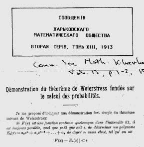
In 1912 Sergei Bernstein introduced his famous polynomials to prove the Weierstrass Approximation theorem:

If \( F(x) \) is any continuous function in the interval [0,1], it is always possible, regardless how small \( \varepsilon \), to determine a polynomial \( E_n(x) = {a_0 x^n + a_1 x^{n-1} + \cdots + a_n} \) of degree \( n \) high enough such that we have \[ {|F(x) - E_n(x)|} < \varepsilon \] for every point in the interval under consideration.

Weierstrass proved the theorem originally in 1885^[1], the very man who had earlier shown how wild a continuous function can be and in particular, how far from being smooth and subject to a Taylor expansion. Bernstein's proof was simple and based on probability theory. Maven Philip J. Davis says that "while [Bernstein's proof] is not the simplest conceptually, it is easily the most elegant".^[2]

Bernstein's 1912 paper^[3] is compact and accessible, at least with some grounding in probability theory. Kenneth M. Levasseur retraces Bernstein more recently in A Probabilistic Proof of the Weierstrass Approximation Theorem^[4] and Wikipedia gives a concise overview of the matter. I propose to follow George Lorentz's approach at the start of his book Bernstein Polynomials^[5], where the basic plan of the proof and the polynomials are retained, but not the overtly probabilistic context.

For a given \( n \geq 0 \), define the \( n + 1 \) Bernstein basis polynomials of degree \( n \) on \( [0, 1] \) as:

\[ B_{k,n}(x) = {{n \choose k}x^k{(1 - x)}^{n-k}}, \hskip{30pt} k = {0, 1, 2, \cdots n}. \]

There are four of them for \( n = 3 \), for example:

\[ B_{0,3} = {(1 - x)}^3, \;\;\; B_{1,3} = 3x{(1 - x)}^2, \;\;\; B_{2,3} = 3x^2(1 - x), \;\;\; B_{3,3} = x^3. \]

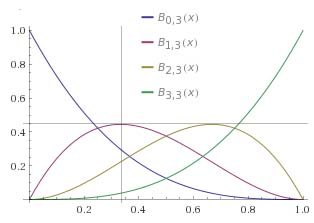
The Bernstein basis polynomials have a number of special properties. They can be used as weighting factors in various contexts due to the key property that for a given \( n \) and any \( x \in [0, 1] \), they all add up to \( 1 \) by the Binomial Theorem:

\[ {\sum_{k=0}^n B_{k,n}}(x) = {(x + (1-x))^n} = 1. \]

Here are the Bernstein basis polynomials for \( n = 3 \), showing an obvious symmetry based on the interplay of \( x \) and \( 1 - x \) in their definitions. The maximum for the \( k^{th} \) one occurs at \( x = k/n \) — the maximum of \( B_{1,3} \) occurs at \( x = 1 / 3 \), for example, as suggested by the crosshairs. As \( n \) increases and there are more of them to sum to \( 1 \) at every point, they drop down closer to the \( x \)-axis, but in such a way as to concentrate mass at the maximum point and tail off rapidly from that point. Plotting them all for larger \( n \) shows a series of hills marching across from left to right, dipping a bit when approaching \( x = 1/2 \), then increasing again.

Since 1960 or so, Bézier curves have been heavily used in computer graphics — they are parametric curves defined in terms of the Bernstein basis polynomials. Given \( n + 1 \) points in the plane \( P_0, P_1, \cdots P_n \), the \( n{th} \) degree Bézier curve determined by the \( P_k \) is:

\[ B(t) = {\sum_{k=0}^n B_{k,n}(t) \cdot P_k}, \hskip{12pt} 0 \leq t \leq 1. \]

Think of the \( P_k \) as vectors, with the \( x \) and \( y \) coordinates being calculated separately. Quadratic and cubic Bézier curves are the most common in practice. The cubic Bézier curve determined by the points \( P_0, P_1, P_2, P_3 \), for example, is:

\[ \begin{align*}
B(t) &= {B_{0,3}(t) \cdot P_0 + B_{1,3}(t) \cdot P_1 + B_{2,3}(t)\cdot \cdot P_2 + B_{3,3}(t) \cdot P_3} \\
&= {{(1-t)}^3 \cdot P_0 + 3t{(1-t)}^2 \cdot P_1 + 3t^2(1-t) \cdot P_2 + t^3 \cdot P_3}.
\end{align*} \]

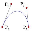
The \( P_k \) in these diagrams are the larger red dots, with \( P_0 \) at the lower left and proceeding clockwise. The Bézier curve goes through \( P_0 \) and \( P_3 \), but not \( P_1 \) and \( P_2 \). The vectors extending from \( P_0 \) to \( P_1 \) and from \( P_3 \) to \( P_2 \) are called handles and can be manipulated in graphics programs like Photoshop to change the shape of the curve, as emulated in the image on the right functioning like a mini pen tool. The handles are tangent to the curve at \( P_0 \) and \( P_3 \) respectively and their length is proportional to how closely the curve follows the handle and for how long. The tangency property is key, causing two Bézier curves stitched together at an endpoint to be smooth at the point of juncture if their respective handles proceed in diametrically opposite directions, \( 180° \) apart (that is, if they lie along the same straight line but proceed in opposite directions).

The Bézier curve is in blue above, the framing straight lines in the diagram on the right being auxiliary. The black dots are at the midpoints of their lines and that frame is built up systematically starting with the outer frame, then the inverted V, and finally the near-horizontal segment riding above the curve. Its midpoint is on the curve and in fact is the point \( B(1/2) \). The left half of the original Bézier curve is itself a Bézier curve determined by \( P_0 \), the original curve's midpoint, and the two black dots towards the left determined by the halving approach. Similarly for the right half of the original Bézier curve. These facts lead to a recursive strategy for rendering Bézier curves known as the De Casteljau algorithm, a truly beautiful bit of software engineering rarely implemented in applications today because Bézier drawing is commonly built into modern APIs (the Bézier curve here was drawn with one line of html5 canvas Javascript — bezierCurveTo()). Drag any of the red points to see the curve and auxiliary lines readjust on the fly (source here).

Approximating a quarter circle with a Bézier curve.

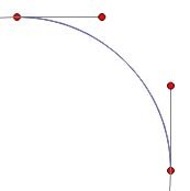
My old article TrueType Font Secrets may be of interest, explaining how TrueType glyphs are made up of quadratic "QSplines", just quadratic Bézier curves stitched together as shown in the case of the outer outline (glyph) of a Times New Roman capital A. Pierre Bézier adapted these curves to be used in CAD programs, but they spread well beyond that. Adobe's use of them in Postscript, PDF, and Photoshop diffused the technology broadly. Evidently even circles are drawn with Bézier curves in Postscript. The image here shows a quarter circle being approximated by a Bézier curve; the fit is not exact, but is off by no more than three parts in 10,000, good enough for all but the most demanding tasks (here is a C program explaining the fit and showing how close it is).

For a given continuous function \( f \) on \( [0, 1] \), the Bernstein polynomial of degree \( n \) for that function is defined in terms of the Bernstein basis polynomials as:

\[ B_n(f)(x) = {\sum_{k=0}^n f\left({k \over n}\right) B_{k,n}(x)} = {\sum_{k=0}^n f\left({k \over n}\right) {{n \choose k}x^k{(1 - x)}^{n-k}}}. \]

To get some grip on what this means for a given \( n \), fix \( x \) and move up the vertical line at \( x \); that line intersects each of the Bernstein basis polynomials of degree \( n \) and as mentioned, the sum of those ordinates is \( 1 \). But think of those values as arrayed along the \( x \)-axis instead of the \( y \)-axis and multiply them one after the other by the equally spaced functional values \( f(k / n) \) for \( k = 1, 2, 3, \cdots n \). In other words, apply the Bernstein values at \( x \) as weighting factors to all the spread-out functional values along the \( x \)-axis.

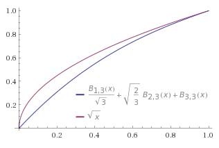
Perhaps a worked example will help show how Bernstein polynomials are constructed. Let \( f(x) = \sqrt{x} \) and \( n = 3 \). Then:

\[ \begin{align*}
B_n(f) = {B_3(\sqrt{x})} &= {\sum_{k=0}^3 \sqrt{{k / 3}} {{3 \choose k}x^k{(1 - x)}^{3-k}}} \\
&= 0 + \sqrt{1/3} {3 \choose 1} x {(1 - x)}^2 + \sqrt{2/3} {3 \choose 2} x^2 {(1 - x)} + \sqrt{3/3} {3 \choose 3} x^3 \\
&= 3 \sqrt{1/3} x {(1 - x)}^2 + 3 \sqrt{2/3} x^2 {(1 - x)} + x^3
\end{align*} \]

Multiplying out and collecting terms:

\[ \begin{align*}
{B_3(\sqrt{x})} &= {(\sqrt{3} - \sqrt{6} + 1) x^3 + (-2 \sqrt{3} + \sqrt{6}) x^2 + \sqrt{3} x} \\
&= 0.28 x^3 -1.01 x^2 + 1.73 x
\end{align*} \]

The image above shows the graphs of \( f(x) = \sqrt{x} \) and \( B_n(f) = B_3(\sqrt{x}) \). The linear term of \( B_3(\sqrt{x}) \) dominates, but higher order terms pull it up a bit towards \( \sqrt{x} \). \( f(x) \) and \( B_n(f) \) agree at \( x = 0 \) and \( x = 1 \), and that is always the case. As \( n \) increases, the \( B_n(f) \) approach \( f \) more closely in a uniform way, that is Bernstein's result.

The \( k^{th} \) Bernstein basis polynomial peaks at \( x = k/n \) and its mass is concentrated there, implying that the greatest contribution to the weighted average constituting the Bernstein polynomial in that vicinity is made by the summands where \( k / n \) is closest to \( x \). This fact plays an important part in proving that \( {\displaystyle \lim_{n \rightarrow \infty}} B_n(f)(x) = f(x) \) and that the convergence is uniform. Bernstein's basic idea is as follows: for a given \( x \), break \( [0, 1] \) into two parts and show that \( |B_n(f)(x) - f(x)| \) can be made small on each one:

1) The subinterval around \( x \) where \( |x - k/n| \) is small.

2) The subintervals to the left and right of (1), where \( |x - k/n| \) is large.

For subinterval (1), only the uniform continuity of \( f \) is used. Subintervals (2) are handled by appealing to properties of the Bernstein polynomials and the binomial coefficients. If \( x = p \) is the probability of an event, then \( B_{k,n}(p) \) is the probability that the event occurs exactly \( k \) times in \( n \) Bernoulli trials. This was Bernstein's take-off point and he cited Bernoulli's probabilistic results to crimp the \( B_{k,n}(p) \) in subintervals (2). The crimping is addressed below without appeal to probability theory in a way that is equivalent to Bernoulli's Weak Law of Large Numbers.

This modest "absorption" identity on binomial coefficients is involved in what follows:

\[ \begin{equation}{{k {n \choose k}} = {n {{n-1} \choose {k-1}}}.} \tag{0} \end{equation} \]

Putting \( n = 5, k = 2 \), for example, leads to \( {{2 {5 \choose 2}} = {5 {4 \choose 1}}} \), or \( {2 \cdot 10} = {5 \cdot 4} \). The absorption identity is easily proved by writing each side in terms of factorials. The following are key:

\[ \begin{equation}{{\sum_{k=0}^n B_{k,n}}(x) = 1.} \tag{1} \end{equation} \]

\[ \begin{equation}{{\sum_{k=0}^n k \cdot B_{k,n}}(x) = nx.} \tag{2} \end{equation} \]

\[ \begin{equation}{{\sum_{k=0}^n k (k - 1) \cdot B_{k,n}}(x) = n(n-1)x^2.} \tag{3} \end{equation} \]

(1) was mentioned above. (2) is proved as follows:

\[ \begin{align*}{\sum_{k=0}^n k \cdot B_{k,n}}(x) &= {\sum_{k=0}^n k {n \choose k} x^k {(1 - x)}^{n - k}} \\
&= {\sum_{k=1}^n n {{n-1} \choose {k-1}} x^k {(1 - x)}^{n - k}} \\
&= n \cdot {\sum_{j=0}^{n-1} {{n-1} \choose j} x^{j+1} {(1 - x)}^{(n-1) - j}} \\
&= nx \cdot {\sum_{j=0}^{n-1} {{n-1} \choose j} x^j {(1 - x)}^{(n-1) - j}} \\
&= {nx \cdot B_{j,{n-1}}(x)} = {nx \cdot 1} = nx. \end{align*} \]

The second line follows from the absorption identity; the indexing is also set to start at \( k=1 \) there because the \( 0^{th} \) term is itself \( 0 \). \( n \) is pulled outside the sum in the third line and sum is re-indexed with \( j = {k-1} \). \( x \) is pulled outside the sum in the fourth line, but then the sum is just \( B_{j,{n-1}}(x) \), which is \( 1 \). (3) is proved similarly using absorption twice. In light of (1) - (3):

\[ \begin{align*}
{\sum_{k=0}^n {(k - nx)}^2 B_{k,n}(x)} &= {\sum_{k=0}^n \{k(k - 1) - (2nx - 1)k + n^2 x^2\} B_{k,n}(x)} \\
&= {n (n - 1) x^2 - (2nx - 1) nx + n^2 x^2} \\
&= {nx(1 - x)} \leq {1 \over 4} n.
\end{align*} \]

The inequality at the last step is because \( x(1 - x) \leq 1/4 \) on \( [0, 1] \). Divide this inequality by \( n^2 \), moving the \( n^2 \) inside the square in the sum on the left to obtain:

\[ {\sum_{k=0}^n {\left({k \over n} - x\right)}^2 B_{k,n}(x)} \leq {1 \over 4n}. \]

Next let \( x \in [0, 1] \) and \( \delta > 0 \), and consider the sum of all \( B_{k,n}(x) \) with \( k \) such that \( |k/n - x| \geq \delta \); that is, where \( k/n \) is bounded away from \( x \):

\[ {\sum_{k \; : \; |k/n - x| \geq \delta} B_{k,n}(x)} \leq {{1 \over \delta^2}\sum_{k \; : \; |k/n - x| \geq \delta} {\left({k \over n} - x\right)}^2 B_{k,n}(x)} \leq {{1 \over \delta^2} \cdot {1 \over {4n}}}. \]

This inequality is true only for \( k \) such that \( |k/n - x| \geq \delta \). For those \( k \), \( {|k/n - x| / \delta} \geq 1 \) and therefore \( {(k/n - x)^2 / \delta^2} \geq 1 \), justifying the introduction of \( (k/n - x)^2 \) and \( \delta^2 \) in the inequality. So if \( |f(x)| < M \) on \( [0, 1] \), then

\[ \begin{equation}{
{\left|f(x) - {\sum_{|k/n - x| \geq \delta} f\left({k \over n}\right) B_{k,n}(x)}\right|} \leq {\sum_{|k/n - x| \geq \delta} \left|f(x) - f\left({k \over n}\right)\right| B_{k,n}(x)} < {2M \over {4 \delta^2 n}} = {M \over {2 \delta^2 n}}.
} \tag{4} \end{equation} \]

(4) holds only for \( k \) with \( |k/n - x| \geq \delta \).

For \( k \) with \( k/n \) closer to \( x \), the uniform continuity of \( f \) can be used as follows. Let \( \epsilon \) be given and choose \( \delta \) such that \( {|f(u) - f(v)|} < \epsilon/2 \) when \( {|u - v|} < \delta \) throughout \( [0, 1] \). So for \( k \) with \( |k/n - x| < \delta \):

\[ \begin{equation}{
{\left|f(x) - {\sum_{|k/n - x| < \delta} f\left({k \over n}\right) B_{k,n}(x)}\right|} \leq {\sum_{|k/n - x| < \delta} \left|f(x) - f\left({k \over n}\right)\right| B_{k,n}(x)} < {\epsilon/2 \cdot 1} = \epsilon/2.
} \tag{5} \end{equation} \]

In plain English, the functional arguments are close together in this range, therefore the functional values are; furthermore, the \( B_{k,n}(x) \) all sum to \( 1 \), so the sum of some of them will be less than that.

The theorem follows by combining (4) and (5). To spell it out, let \( \epsilon > 0 \) be given and choose \( \delta \) so that (5) holds, as discusssed above. Then for that \( \delta \), choose \( n \) high enough so that \( {M / {(2 \delta^2 n)}} < {\epsilon / 2} \) and the left side of (4) is less than \( \epsilon / 2 \). It follows that for all \( x \) in \( [0, 1] \):

\[ {\left|f(x) - {\sum_{k=0}^n f\left({k \over n}\right) B_{k,n}(x)}\right|} < {\epsilon / 2 + \epsilon / 2} = \epsilon. \]

QED.

Mike Bertrand

March 17, 2015

^ 1. Über die analytische Darstellbarkeit sogenannter willkürlicher Functionen einer reellen Veränderlichen (About the analytic representation of so-called arbitrary functions of one real variable), by Karl Weierstrass, Sitzungsberichte der Königlich Preußischen Akademie der Wissenschaften zu Berlin, 1885, II (p. 633).

^ 2. Approximation and Interpolation, by Philip J. Davis (Dover Publications, 1975), ISBN 3-486-62495-1. Originally published in 1963. "while [Bernstein's proof] is not the simplest conceptually", p. 108.

^ 3. Démonstration du théorème de Weierstrass fondée sur le calcul des probabilités (Demonstration of a theorem of Weierstrass based on the calculus of probabilities), by Sergei Bernstein, Communications of the Kharkov Mathematical Society, Volume XIII, 1912/13, p. 1-2. English translation.

^ 4. "A Probabilistic Proof of the Weierstrass Approximation Theorem", by Kenneth M. Levasseur (The American Mathematical Monthly, Vol 91, No 4, April 1984, pp. 249-250).

^ 5. Bernstein Polynomials, by G. G. Lorentz (Chelsea Publishing Company, 1986), ISBN 978-0-8218-7558-2. Originally published in 1953.