Argand Proves the Fundamental Theorem of Algebra

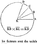
Complex multiplication in Argand (Essai, 1806).
The Fundamental Theorem of Algebra states that every non-constant polynomial with complex coefficients has at least one root in the complex plane. The quadratic formula provides two roots for every complex quadratic polynomial, considering that every complex number has two square roots. There are similar formulas for polynomials of degree three and four, but no general formula for polynomials of degree higher than that. This theorem has a long pedigree going back to Euler and before, d'Alembert attempting a proof in 1748. Gauss is often credited with the first proof in 1799, but it was incomplete.[1] Argand gave a simple and direct proof in 1806 in an anonymous self-published pamphlet where he showed how to represent complex numbers geometrically and took up complex addition, multiplication, division, root taking, and absolute value.[2]
This theorem played a key role in the development of complex numbers considering their intimate connection with solving polynomial equations, an intense interest of mathematicians since the sixteenth century. Reinhold Remmert puts it this way:
The fundamental theorem of algebra is of outstanding significance in the history of the theory of complex numbers because it was the possibility of proving this theorem in the complex domain that, more than anything else, paved the way for a general recognition of complex numbers.[2a]
Argand's proof too was incomplete, wanting only verification of the fact that the absolute value of a complex polynomial assumes an absolute minimum in the complex plane (he considered this axiomatic). He expanded the skeletal proof of 1806 in an article in 1815, "Reflexions sur la nouvelle théorie des imaginaires, suivies d'une application à la démonstration d'un théorème d’analise" ("Reflections on the new theory of imaginaries, followed by an application to the demonstration of a theorem of analysis"). I take up his proof of the Fundamental Theorem of Algebra in "Reflexions" in this article — see my translation of "Reflexions" to English.[3]
Representing Complex Numbers Geometrically
Jean Robert Argand is one of the great amateurs in the history of mathematics but not much is known about him. He was one of the first to show how to represent complex numbers as points in the plane and his exposition of 1806 was correct and thorough-going — it could have been written yesterday with little change, testifying to how very right he was. Argand presented his simple proof of the Fundamental Theorem of Algebra as evidence for the efficacy of his method, writing that other proofs may be available, but that the geometric approach made it easier and more accessible. Cauchy made the point decisively by dressing up Argand's proof only to obscure the underlying principles.
Argand wrote that directed lines (lignes dirigées) in the plane can represent complex numbers, where \(\sqrt{-1}\) is represented by the vertical line from \((0,0)\) to \((0,1)\) and every other complex number is represented by a directed line from the origin to some point in the plane, as is now familiar. He didn't use \(i\) for the imaginary unit and warned against reading too much into the term "imaginary", his entire enterprise giving consistent, concrete meaning to complex numbers. He gave the parallelogram law for adding complex numbers and explained how complex numbers along the unit circle are multiplied by adding their angles, scaling being applied for complex numbers not on the unit circle. He gave the familiar rules for negation, dividing, taking roots, and calculating the absolute value.
Plan of the Proof
Argand's proof depends on the facts that:
1) The absolute value of a complex polynomial assumes its absolute minimum in the complex plane; that is, there is a point \(z_m \in \mathbb{C}\) such that \(|f(z_m)| \leq |f(z)|\) for all \(z \in \mathbb{C}\).
2) Argand's Inequality: For every non-constant \( f(z) \in \mathbb{C}[x]\) and every point \(z \in \mathbb{C}\) such that \(|f(z)| \neq 0\), there is a point \(z_0\) close to \(z\) such that \(|f(z_0)| < |f(z)|\).
The proof of the Fundamental Theorem follows directly from (1) and (2). For suppose \(f(z)\) is a non-constant complex polynomial and \(|f(z_m)| \leq |f(z)|\) for all \(z \in \mathbb{C}\). Suppose further that \(f(z_m) \neq 0\), so of course \(|f(z_m)| \neq 0\) as well. Then by (2), there is a point \(z_0\) close to \(z_m\) such that \(|f(z_0)| < |f(z_m)|\). This contradicts the minimality of \(z_m\), so it must be true that \(|f(z_m)| = 0\) and consequently \(f(z_m) = 0\). That is, \(z_m\) is a root of \(f(z)\).
Argand took (1) for granted, though it is far from obvious and wasn't proven satisfactorily until later. His proof rests on (2), which he demonstrated with admirable clarity, a proposition Remmert calls "Argand's Inequality".[4] (1) can be derived from two other facts:
1') A non-constant complex polynomial is unbounded away from the origin, matching a theorem for real polynomials. That is, given \(M > 0\), there is an \(N > 0\) such that \(|f(z)| > M\) for all \(|z| > N\).
1'') The absolute value of a complex polynomial assumes an absolute minimum on a compact subset of the complex plane. That is, if \(f(z) \in \mathbb{C}[x]\) and \(K\) is a compact subset of \(\mathbb{C}\), then there is a \(w \in K\) such that \(|f(w)| \leq |f(z)|\) for all \(z \in K\).
(1') is an natural generalization of the situation for a real non-constant polynomial \(g(x),\) where the highest power of \(x\) eventually dominates and drives \(g(x)\) to \(\pm \infty\) as \( x \longrightarrow \pm \infty.\)
(1'') is a form of the Extreme Value Theorem, proven for real functions by Bolzano in 1830, but which went unrecognized until Weierstrass's much later work.[5]
Argand's Inequality
Argand's proof depends on:
Theorem. For every non-constant \( f(z) \in \mathbb{C}[x]\) and every point \(z \in \mathbb{C}\) such that \(|f(z)| \neq 0,\) there is a point \(z_0\) close to \(z\) such that \(|f(z_0)| < |f(z)|\).
Proof. Let \(z\) be a complex number such that \(|f(z)| \neq 0.\) It suffices to prove the theorem for monic polynomials, so let \(f(z) = z^n + a_{n-1} z^{n-1} + a_{n-2} z^{n-2} + a_1 z + a_0,\) where \(n \geq 1\) and the \(a_i\) are complex. Let \(h\) be a complex increment[6] and expand \(f(z+h)\) to give:
\begin{align}
f(z+h) = f(z) &+ \left\{nz^{n-1} + (n-1)a_{n-1}z^{n-2} + \cdots + a_1\right\}h\\
&+ \left\{{n \over 1} \cdot {{n-1} \over 2}z^{n-2} + \cdots \right\}h^2\\
&\vdots\\
&+ \left\{nz + a_{n-1}\right\}h^{n-1}\\
&+ h^n.
\end{align}
Since some of those expressions in the curly braces can be zero, complicating the argument, rewrite this equation as:
\[f(z+h) = f(z) + Rh^r + Sh^s + \cdots + Vh^v + h^n,\tag{1}\]
where none of the coefficients \(R, S, \cdots V\) are zero and the exponents of \(h\) are whole numbers strictly increasing from left to right: \(1 \leq r < s < \cdots < v < n.\)
Note that if all the coefficients \(R, S, \cdots V\) were zero, then (1) would reduce to \(f(z+h) = f(z) + h^n\) and then putting \(h = \sqrt[n]{-f(z)}\) gives \(f(z+h) = 0,\) so the theorem would be proven for this case, which can therefore be ignored in what follows. Thus we can assume that \(R \neq 0.\) The object is to choose the direction and length of \(h\) so that \(|f(z+h)| < |f(z)|,\) that is, so that \(f(z+h)\) is closer to the origin than \(f(z)\) is.

Direction of \(h\). Choose \(h\) so that the direction of \(Rh^r\) is diametrically opposite to the direction of \(f(z),\) thought of as a vector emanating from the origin and ending at complex number \(f(z)\) in the plane. The point of this choice is that \(f(z)\) and \(Rh^r\) will have an offsetting effect on the right hand side of (1).
Length of \(h\). Choose \( h\) so that its length is less than one, less than the length of \(f(z)\) and also such that:
\[|Sh^s + \cdots + Vh^v + h^n| < |Rh^r|.\tag{2}\]
To see that this is always possible, let \(D = Sh^s + \cdots + Vh^v + h^n\) be the vector on the left side of (2) and note that:
\begin{align}
|D| &= |Sh^s + \cdots + Vh^v + h^n|\\
&\leq |Sh^s| + \cdots + |Vh^v| + |h^n|\\
&= |S| \cdot |h|^s + \cdots + |V| \cdot |h|^v + |h|^n\\
&< |R| \cdot |h|^r.
\end{align}
The last inequality holds because there are a fixed number of summands and the exponents on the previous line (\(s, v, \cdots n)\) are all strictly greater than \(r,\) so \(|h|^s\) is dominated by \(|h|^r\) and so are the other powers of \(|h|,\) all the more so because their exponents are strictly greater than \(s.\) To put it analytically, the following two statements are equivalent, the second derived from the first by dividing by \(|h|^r\):
\begin{align}
|S| \cdot |h|^s + \cdots + |V| \cdot |h|^v + |h|^n &< |R| \cdot |h|^r\\
|S| \cdot |h|^{s-r} + \cdots + |V| \cdot |h|^{v-r} + |h|^{n-r} &< |R|,\\
\end{align}
and the expression on the left of the second inequality can be made as small as desired by choosing \(|h|\) small enough. Argand explicitly states that \(|pq| = |p|\cdot |q|\) and plainly relies on the triangle inequality, writing of des premiers élémens de géométrie (the first elements of geometry) and of how \(f(z+h)\) sera représenté par la ligne brisée ou droite (will be represented by a broken or straight line).
The geometry in question is illustrated by the diagram, which Argand recommends drawing : J'inviterai le lecteur à tracer une figure, pour suivre cette démonstration (I invite the reader to draw a figure to follow this demonstration). The long diagonal vector from the origin points to \(f(z)\) and vector \(Rh^r\) is an increment pointing in the diametrically opposite direction. Add vector \(D\) to that to arrive at point \(f(z+h),\) which lies on the small red circle, which is strictly contained in the large circle centered at the origin going through \(f(z).\)
To nail it down, let \(Rh^r = -tf(z),\) where \(0 < t < 1.\) Then starting with (1):
\begin{align}
|f(z+h)| &= |f(z) + Rh^r + Sh^s + \cdots + Vh^v + h^n|\\
&\leq |f(z) + Rh^r| + |Sh^s + \cdots + Vh^v + h^n|\\
&=|f(z) + Rh^r| + |D|\\
&< |f(z) + Rh^r| + |R| \cdot |h|^r\\
&= |f(z) - tf(z)| + |R| \cdot |h|^r\\
&= (1 - t)|f(z)| + |R| \cdot |h|^r,\\
\end{align}
where the first summand on the last line is always strictly less than \(|f(z)|\) and the second summand, although positive, can be made as small as desired. It follows that there is a complex increment \(h\) such that \(|f(z+h)| < |f(z)|.\) QED.
Basins of Attraction and the Julia Set
Let \(\alpha\) be a root of \(p(x) \in \mathbb{C}[x].\) Then:
\[p(x) = (x - \alpha)q(x),\]
where \(q(x)\) is a complex polynomial with degree one less than that of \(p(x).\) Argand's proof shows that \(q(x)\) too has a root, and the process can be continued to completely factor \(p(x):\)
\[p(x) = (x - \alpha_1)(x - \alpha_2)(x - \alpha_3) \cdots (x - \alpha_n),\]
where the \(\alpha_i\) are exactly the roots of \(p(x).\) So a complex polynomial of degree \(n\) has exactly \(n\) roots.
Argand's method can be used to find roots as well. His equations (1) and (2) are the Taylor expansions of \(f\) around \(z\) and can be written:
\[ f(z+h) = f(z) + f'(z) \cdot h + {f''(z)\over 2!} \cdot h^2 + {f'''(z) \over 3!} \cdot h^3 + \cdots.\]
Assume \(f'(z) \neq 0,\) so \(Rh^r = f'(z) \cdot h\) in Argand's derivation. Assume further that \(z_0 = z\) and \(z_1 = z + h,\) so \(h = z_1 - z_0.\) Argand says choose the direction of \(h\) so that the direction of \(Rh^r = f'(z) \cdot h\) has direction opposite that of \(f(z).\) Ignoring the length of \(h,\) this leads to:
\begin{align}
f'(z_0) \cdot h &= -f(z_0)\\
z_1 - z_0 &= h = -{{f(z_0)} \over {f'(z_0)}}\\
z_1 &= z_0 -{{f(z_0)} \over {f'(z_0)}}\tag{3}.
\end{align}

(3) is the formula for Newton-Raphson iteration in the complex plane! Newton-Raphson is a method which, when iterated, usually converges to a root of \(f(z)\) in the complex plane, generalizing the situation for real polynomials. The next step in the iteration of (3) is:
\[z_2 = z_1 -{{f(z_1)} \over {f'(z_1)}},\]
and subsequent \(z_i\) are calculated similarly.
Consider \(f(z) = z^2 - z + 1,\) for example, with roots \(z = (1 \pm \sqrt{3}i) / 2 = 0.5 \pm 0.86603i.\) Putting \(z = z_0\) and \(g(z) = z_1,\) (3) becomes:
| \(k\) | \(z_k\) | \(|f(z_k)|\) |
| 0 | 1.62500 + 2.00000i | 4.91810 |
| 1 | 0.98238 + 1.14243i | 1.14838 |
| 2 | 0.62356 + 0.84980i | 0.21439 |
| 3 | 0.49895 + 0.85704i | 0.01558 |
| 4 | 0.50001 + 0.86607i | 0.00008 |
| 5 | 0.50000 + 0.86603i | 0.00000 |
| 6 | 0.50000 + 0.86603i | 0.00000 |
\begin{align}
g(z) &= z - {{f(z)} \over {f'(z)}}\\[.5em]
&= z - {{z^2 - z + 1} \over {2z - 1}}\\[.5em]
&= {{(2z^2 - z) - (z^2 - z + 1)} \over {2z - 1}}\\[.5em]
&= {{z^2 - 1} \over {2z - 1}}.
\end{align}
So Newton-Raphson iteration for \(f(z)\) consists of choosing an initial point \(z_0\) in the complex plane and repeatedly iterating \(g(z)\) starting with \(z = z_0.\) The image and chart show the Newton-Raphson iteration for \(f(z)\) starting at \(z_0 = 1.625 + 2i,\) out of sight up and to the right. The \(z_i\) converge rapidly to the root in the first quadrant, agreeing with the root to five places starting at \(z_5.\) Note that \(|f(z)|\) decreases at every step, and rapidly so.
If \(z_0\) is real, then all subsequent values in the iteration are real as well, so Newton-Raphson does not converge to a root for starting points \(z_0\) along the \(x-\)axis, and in fact such sequences do not converge at all. But starting at any other point in the complex plane does result in convergence to one of the roots. In fact, the \(z_i\) converge to the root in the first quadrant if \(z_0\) is in the upper half-plane, like in this example, while convergence is to the root in the fourth quadrant if \(z_0\) is in the lower half-plane. This effect, convergence for all points except along a line intermediate between the two roots, holds for all complex quadratic polynomials.
The upper half-plane in this example is a basin of attraction of \(g(z),\) as is the lower half-plane. The line between them, the boundary of each, is the Julia set of \(g(z).\) The predictability and good behavior of points iterated starting from a point in a basin of attraction contrasts with the chaotic behavior of points iterated starting from the Julia set, which do not converge and oscillate wildly. No matter how closely two points are in the Julia set, their iterates eventually diverge from each other. And of course a Julia point and nearby basin point share different fates when iterated. Compare the trajectories of \(z_0 = 10 + 0i\) and \(w_0 = 10 + 0.01i\) when iterating \(g(z),\) for example: two close points, but one in the Julia set and one in a basin. Iterates of \(z_0\) oscillate crazily back and forth on the \(x-\)axis, while iterates of \(w_0\) hover just above the axis, always in the basin, but moving towards the origin, and eventually arcing up to the root.
From Argand to Fractals
The foregoing applies to the polynomial \(f(z) = z^2 - z + 1,\) but is characteristic of any quadratic complex polynomial. However, the situation becomes much more complex for polynomials of degree three and higher.
Consider \(f(z) = z^3 - 1,\) an ostensibly straightforward example. The roots are the cube roots of unity: \(z = 1, (- 1 \pm \sqrt{3}i)/2\) and the corresponding Newton-Raphson function is:
\[g(z) = {{2z^3+1} \over {3z^2}}.\tag{4}\]
Iterating \(g(z)\) starting at most points in the plane converges to one of the roots, tempting one to guess there is a nice symmetric three-way division of the plane defining the basins of attraction. Not even close! Symmetry there is, but of a more complex form, with each basin of attraction spread all over the plane in enticing fractal florets.[7] This image shows the three basins of attraction colored depending on the root each converges to, the black points indicating the three roots.

Basins and Julia Set for \(z^3 - 1 = 0.\) Black dots are the cube roots of unity.
Let \(z_0\) be a point in the plane where iteration starts. Any \(z_0\) in the red third-plane to the right converges to \(z = 1\) when iterated. It's not exactly a third-plane because multicolored bites are taken out along the diagonal lines \(y = \sqrt{3}x\) up and to the right and \(y = -\sqrt{3}x\) down and to the right. So not exactly a third-plane, but close and all seeming reasonable. Less expected are the red regions scattered throughout the plane. Almost all points along the negative \(x-\)axis are red, for example, the exceptions being the white points at the intersections of the floret-like structures stretching along the axis to the left. \(g(-{1 \over 2}) = 1,\) for example, one iteration leading to the root. Similarly for \(z_0 = -{1 \over 8},\) though the convergence is slower — \(g(-{1 \over 2}) = 21.25, g(21.25) = 14.167,\) and so on, converging down to \(1.\)

Floret in \(z^3-1=0\) fractal.
The white points along the negative \(x-\)axis are in the Julia set; there are a denumerably infinite number of them at the intersections of the florets. The first one is \(w_0 = -\sqrt[3]{1 \over 2} = -0.793700526.\) To see this, note that \(g(w_0)=0, g(0)=\infty, g(\infty)=\infty,\) so there is no convergence to a root.[8] Back-calculating from (4), the next Julia point out along the negative \(x-\)axis is:
\[w_0' = -{{1+\sqrt[3]{5-2\sqrt{6}} + (5-2\sqrt{6})^{2/3}} \over {2 \sqrt[3]{2} \sqrt[3]{5-2\sqrt{6}}}} = -1.433775499.\]
By the way it was calculated, \(g(w_0') = w_0\) and further iterations proceed as before. Iterating from any of those Julia points out the negative \(x-\)axis results in values skipping to the right visiting each floret intersection and eventually veering to infinity after getting to \(w_0.\)
The white points constitute the Julia set, each point of which borders all three basins. The origin is typical of a Julia point, bordered by each basin from two different directions directly opposite each other. Which basin depends on which \(120^\circ\) sector the point is in, no matter how how close that point is to the origin. Staring at the vicinity of the origin, it seems that lines of white emanate from it, but that's just due to reaching the resolution of the device displaying those pixels. Zooming in would show that every one of the white points is the intersection of two florets like \(w_0\) is. That is characteristic of fractals, that the appearance at different resolutions is similar or identical.
Choosing a \(z_0\) along the negative \(x-\)axis but not a Julia point (that is, in the red portion of one of the florets to the left) results in the iterated points hop-scotching to the right, visiting a new floret each time, then jumping to the positive \(x-\)axis and from there converging to \((1,0).\) Consider \(z_0 = (-2,0),\) for example, where the iterates start marching to the right one floret at a time, then jump over to the positive side to a point between \(0\) and \(1,\) next to a value greater than \(1,\) and from there start converging monotonically down to \(1:\)
\[-2 \rightarrow -1.25 \rightarrow -0.62 \rightarrow 0.453819 \rightarrow 1.92105 \rightarrow 1.37102 \rightarrow 1.09135 \rightarrow 1.00743\]

Iterate in the blue basin.
By the definition of a basin, all iterates have the same color as the initial point. Starting with \(z_0\) anywhere in a blue region will result in iterates always in the blue, for example. Take the blue point \( z_0 = -0.68282 + 0.154185,\) as pictured here. The first iterate \(z_1\) is in the blue part of the big floret immediately up and to the right of the origin. The second iterate \(z_2\) is in the unbounded blue region down and to the left, and subsequent iterates converge to the root in the blue region.
The original image suggests three-fold symmetry around the origin and this is indeed the case. That is, rotating the image counter-clockwise by \(120^\circ\) results in the same image with red \(\rightarrow\) green \(\rightarrow\) blue \(\rightarrow\) red. This follows from the fact that \(g(\xi z) = \xi \cdot g(z),\) where \(\xi = \cos{120^\circ} + i \sin{120^\circ},\) the value which rotates a complex number counter-clockwise around the origin by \(120^\circ\) when multiplied by that complex number:
\begin{align}
g(\xi z) &= {{2(\xi z)^3+1} \over {3(\xi z)^2}}\\[.5em]
&= {{\xi^3 \cdot 2z^3+1} \over {\xi^2 \cdot 3z^2}}\\[.5em]
&= {{2z^3+1} \over {\xi^2 \cdot 3z^2}}\\[.5em]
&= \xi \cdot {{2z^3+1} \over {\xi^3 \cdot 3z^2}}\\[.5em]
&= \xi \cdot {{2z^3+1} \over {3z^2}}\\[.5em]
&= \xi \cdot g(z).
\end{align}
The cancellations are because \(\xi^3=1\). To understand this, start with a point \(z_0\) somewhere in the infinite part of the red basin off to the right. Iterating \(g(z)\) starting with \(z_0\) is matched point for point by a sequence in the infinite part of the green basin, each green point being the rotated correspondent of a red point. Just as the red points converge to 1, so too the green points converge to \((-1+\sqrt{3}i)/2.\) The effect is the same for any point in the plane, noting only that there will be no convergence for either point if the original point is in the Julia set (so the rotated one is too).
Argand's Legacy

Argand's Essay of 1806
Argand's article of 1806 was self-published and anonymous. Very little is known about him, even whether Argand was his real name or a pseudonym. The St. Andrews account of Argand is the most thorough I've seen, emphasizing that the Jean-Robert Argand found in the historical record, obscure as he was, may not be our mathematician.
Leading mathematicians ignored Argand (or pretended to) for fifty years and more while systematically integrating his ideas into the fabric of mathematical practice. Cauchy's article of 1820, "Sur les racines imaginaires des équations" followed Argand's proof closely if ham-handedly, allowing only for real polynomial coefficients and pressing real increments \(h\) and \(k\) into service, generally beating Argand's elegant geometric approach into a more conventional exercise in trigonometry (preferable however to the exhausting and truly grim account in his influential textbook of 1821, Cours d'analyse.[9] All without so much as a tip of the hat to his prescient but obscure predecessor. Cauchy cited Legendre as inspiration, but I'm guessing the latter's contribution involved forwarding Argand's work rather than writing something about root finding in his Théorie des nombres, as Cauchy claimed.[10]
The case of Gauss is particularly bizarre. He gave many proofs of the Fundamental Theorem of Algebra over a lifetime (the first in his doctoral thesis in 1799), none as direct or elegant as Argand's and some of them just as incomplete. He came out whole-heartedly for using the plane to represent complex values in 1831, but in the context of biquadratic residues, a technical area of number theory. Gauss noticed that results in this area became markedly easier by considering complex numbers with integer components, breaking up the plane in \(1 \times 1\) squares. This system is now known as the Gaussian Integers. His report of 1831[11] was eloquent on the necessity of expanding the integers to the complex (now Gaussian) integers, including:
If one formerly contemplated this subject from a false point of view and therefore found a mysterious darkness, this is in large part attributable to a clumsy terminology. (p. 313)
Yet he is silent on using the plane to represent all complex numbers, the multiplication and root-taking rules, and so on, all addressed by Argand so comprehensively twenty-five years earlier — an inexplicable omission considering his assertion that he'd been thinking along these lines since 1799. He even writes of thinking of \(i = \sqrt{-1}\) as the geometric mean between \(1\) and \(-1,\) just as Argand had in 1806. Again, Argand's name goes unmentioned.
\(\sqrt{-1}\) had been shrouded in mystery and confusion before the Argand diagram, as it is now called. Complex numbers were called "absurd" and "impossible" even when being employed, the term "imaginary" perfectly encapsulating their barely legitimate status. The situation mirrored the earlier uneasiness over negative numbers, but arguably with more justification — what could \(\sqrt{-1}\) possibly mean when everyone knows that squares must be positive. Yet complex numbers gave results, and consistent ones! The Italian algebraists of the sixteenth century would combine complex values to produce real roots, for example. Argand resolved the uneasiness once and for all, giving a consistent, concrete, and intuitive model for complex numbers that was highly productive of new results as well.
Argand wasn't even the first to represent complex numbers geometrically, that honor going to Caspar Wessel, who published a thorough-going account of the geometric approach to complex numbers in Danish in 1799. Wessel's work was truly buried, not being rediscovered until 1895. Wessel was another amateur mathematician, a surveyor by trade, and an accomplished one. Anachronism and Whiggism are always dangerous when thinking retrospectively, but that these brilliant amateurs could see the way so clearly makes the stubborn resistance at the top seem puzzling, Cauchy in particular, a founder of complex function theory, holding out till late in the day.[12]
Argand started to receive recognition as the nineteenth century progressed. J. Hoüel published the original Essai in 1874 and A. S. Hardy brought out an English translation in 1881 under the title Imaginary Quantities: Their Geometrical Interpretation — both these books included valuable commentary and helped secure Argand's reputation and his priority. George Chrystal paid tribute to Argand in England in his influential Algebra, an Elementary Text-Book, whose 5th edition in 1904 followed Argand closely in proving the Fundamental Theorem, fully crediting the old master, whose proof he called "both ingenious and profound" (p. 248).
That notation is critical in mathematics is a long accepted truism. Here we have not only notation, but an entire way of thinking unlocking a whole new world. Argand's proof of the Fundamental Theorem of Algebra demonstrated not only the proposition in question, but even more importantly, the efficacy of this new approach, just as he said.
Mike Bertrand
December 3, 2022
^ 1. See Numbers, by Heinz-Dieter Ebbinghaus, et al., Springer (1991), ISBN 0-387-97497-0. Chapters 3 and 4 by Reinhold Remmert pertain to this story, with Chapter 4 taking up the Fundamental Theorem of Algebra and its deep history. Remmert features Argand's proof (pp. 111-113), which he describes as "possibly the simplest of all the proofs, one based on an old and beautiful idea used by Argand." (p. 98).
^ 2. "Essai sur une manière de représenter les quantités imaginaires, dans les constructions géométriques", by R. Argand, Annales de Mathématiques pures et appliquées, tome 4 (1813-1814), pp. 133-147. Argand self-published the Essai anonymously in 1806. The sketch of the Fundamental Theorem starts on p. 142, where Argand cites it as an application of his method ("Comme application à l’algèbre ..."). An English translation appeared in 1881: Imaginary Quantities: Their Geometrical Interpretation, by A. S. Hardy, D. Van Nostrand (1881).
^ 2a. Numbers, p. 97.
^ 3. "Réflexions sur la nouvelle théorie des imaginaires, suivies d'une application à la démonstration d'un théorème d'analise", by R. Argand, Annales de Mathématiques pures et appliquées, tome 5 (1814-1815), pp. 197-209. English translation.
^ 4. Numbers, p. 112.
^ 5. "Bolzano and uniform continuity", by Paul Rusnock and Angus Kerr-Lawson, Historia Mathematica 32 (2005), pp. 303–311. They state that Bolzano gave a nice proof in 1830 that "a function continuous on a closed interval assumes global maximum and minimum values on the interval". It is a short step from there to the analogous theorem for disks in the plane.
^ 6. Argand uses \(i\) for the complex increment, confusing the modern reader — I use \(h\) instead.
^ 7. A fractal is a geometric shape which is typically similar to itself at different resolutions, or nearly so. Fractals came into prominence through the Mandelbrot set in the 1980s, which is generated by an iterative process in the complex plane similar to that developed in this article.
^ 8. It is customary in this field to extend the complex numbers by adding \(\infty\) — this is the Riemann sphere. For a basic introduction to Julia Sets and how iterative processes in the complex plane produce fractals, see "Cayley's Problem and Julia Sets", by H. O. Peitgen, et al., Mathematical Intelligencer, 6 (1984), pp. 11-20.
^ 9. The Fundamental Theorem of Algebra takes up Chapter X in Cauchy's Cours d'analyse. There is an English translation of the entire book: Cauchy's Cours d'analyse: An Annotated Translation, by Robert E. Bradley and C. Edward Sandifer, Springer Science (2009), ISBN 978-1-4419-0548-2.
^ 10. Argand had given his Essai of 1806 to Legendre, who transmitted it to other mathematicians. See The Higher Calculus: A History of Real and Complex Analysis from Euler to Weierstrass, by Umberto Bottazzini, translated by Warren Van Egmond, Springer-Verlag (1986), ISBN 0-387-96302-2, p. 139. Bottazinni writes that only in 1849 did Cauchy abandon the approach of Cours d'analyse and "finally adhere to the geometrical theory that had been proposed by Argand in 1806, against which, in Cauchy's view, 'specious objections' had been advanced". (p. 168) Bottazzini cites an article of Cauchy, but Gallica has them listed as two separate articles back-to-back: "Mémoire sur les quantités géométriques" and "Méthode nouvelle pour la résolution des équations algébriques". Cauchy credits Argand somewhat grudgingly as one of the authors of the geometric approach, writing of a "méthode nouvelle" (!) in the second article.
^ 11. Gauss's entire report of 1831 is in From Kant to Hilbert, Volume 1: A Source Book in the Foundations of Mathematics, by William Ewald, Oxford University Press (1996), ISBN 0-19-850535-3, pp. 306-313 (including an introduction by Ewald).
^ 12. Two more works appeared in 1828: "A Treatise on the Geometrical Representation of the Square Roots of Negative Quantities", by Rev. John Warren; and "La vraie théorie des quantités négatives et des quantités prétendues imaginaires", by C. V. Mourey. Warren influenced Hamilton and is cited in the latter's work on quaternions. Mourey was self-published and evidently an amateur — he included a proof of the Fundamental Theorem of Algebra (p. 104ff) that Coolidge says "shows a very considerable amount of acumen" (The Geometry of the Complex Domain, by Julian Lowell Coolidge (1924), p. 27).