Descartes and La Géométrie
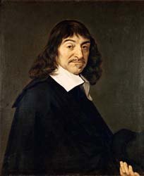
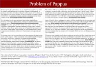
René Descartes in 1648.
Everyone knows that Descartes founded analytic geometry with his little essay La Géométrie, published in 1637 as an appendix and proof-of-concept for a work on philosophy, Discourse on Method. As always, the story is more complex and interesting than that. The canonical modern work in English is History of Analytic Geometry[1] by Carl Boyer, which includes this from his much-admired antecedent Gino Loria (1862-1954):
In truth, whoever studies thoroughly the treatise of Apollonius on Conics must confess the profound analogy it bears to an exposition of the properties of the curves of second degree by means of Cartesian coordinates; not only do the fundamental properties employed by the Greek geometer to distinguish the three curves one from the other translate into the canonical equations of the same in Descartes' method, but many of the reasonings given, when translated into the ordinary language of algebra, answer to elimination, solution of equations, transformation of coordinates, and the like. What we would however seek in vain in the Greek geometer is the concept of a system of axes, given a priori, of the figure to be studied.
The last sentence applies equally well to La Géométrie. To get a sense of Apollonius's bona fides as a precursor of analytic geometry, consider this important theorem of his, used by Newton in the Principia:
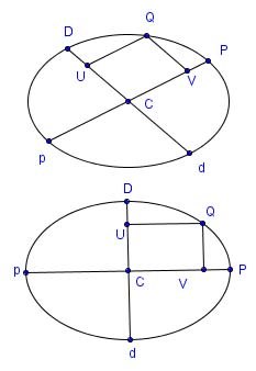
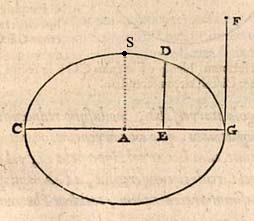
If PCp, DCd be conjugate diameters of an ellipse, and QV an ordinate of Pp, then QV² : PV · Vp :: CD² : CP².
An ellipse diameter is simply a chord through the center, conjugate diameters a pair of them where each is parallel to the tangent at the points on the ellipse cut by the other one. Apollonius and Newton had the top picture in mind, but the theorem applies equally well to the bottom one and here the term "ordinate" is in keeping with modern usage. Apollonius had the concept of ordinate too, but for him it meant a line segment dropped from a point on the ellipse down to a diameter and parallel to that diameter's conjugate (QV in the top picture as well as the bottom one). Rotate all the line segments in the top picture clockwise around center C to produce something like the bottom picture - it's not exact, but helps show the relation between them. To be exact, proceed as follows to transform the top picture into the bottom one:
S1: Scale the top image in x, compressing it until it is a circle fitting snugly inside the original ellipse and with the same center. At that point the conjugate diameters will be perpendicular and ∠UQV 90°.
R1: Rotate clockwise until Pp is horizontal (and Dd is vertical).
S2: Scale again in x, stretching until the ellipse has it's original shape.
Each of these operations is an affine transformation, so their composition \( S2 \circ R1 \circ S1 \) is too. Affine transformations preserve lines, parallelism, the ratio of lengths along a give line, and the ratio of areas. In fact, older geometers would see the theorem as a statement about areas - QV² is literally the area of the square on segment QV, PV · Vp is the area of the rectangle made up of those two segments, and so on.
Let's translate the theorem into the language of modern analytic geometry, using the bottom picture. Let C be the origin with Pp the x axis and Dd the y axis. Q = (x,y) is any point on the ellipse and a = CP and b = CD the semi-axes. Applying Apollonius's theorem:
\[ {a^2 \over b^2} = {CD^2 \over CP^2} = {QV^2 \over {VP \cdot Vp}} = {x^2 \over{(b-y)(b+y)}} = {x^2 \over{b^2-y^2}}. \]
Equating the fractions at start and end, cross-multiplying, and simplifying leads to:
\[ {{x^2 \over a^2} + {y^2 \over b^2}} = 1, \]
the canonical equation of an ellipse in modern analytic geometry. That is, Apollonius's theorem in a rectangular coordinate system is equivalent to the modern equation of an ellipse, and easily proven so. Also, the theorem for rectangular coordinates implies it in all generality. With the figures above, for example, \( {S1 \circ R1 \circ S2} = {(S2 \circ R1 \circ S1)^{-1}} \) is an affine transformation taking the bottom figure into the top one. But the theorem involves ratios of areas, which are preserved by affine transformations, so the theorem applies equally well to the figure with oblique axes. This constitutes a proof of Apollonius's theorem in a modern setting and one that is a whole lot easier than Apollonius's or anyone in his tradition! That's why we like analytic geometry and why Descartes and his followers are important. Still, Apollonius was close, properly understood — that is Loria's point in the quote above.
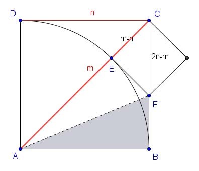
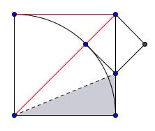
Click image for a geometric proof of the irrationality of \( \sqrt{2} \) (same as the incommensurability of the side and diagonal of a square).
But the discovery of incommensurables turned the Greeks away from uniting geometry and numbers, they favored synthetic geometry determinedly and as a matter of principle (Dirk Struik's Chapter III on the Greeks[2] is illuminating). The Greek numeration system was ineffective and had no place value. They had no algebra to speak of and early Pythagorean efforts emphasizing numbers were consciously aborted. Awakening Europe revered the ancients, but the old texts gave little impetus towards an analytic geometry. Boyer insists (p viii) that the subject developed autonomously, unaffected by broader material and social factors — maybe the pace would have been quickened were it otherwise. Circa 150 AD the geographer Ptolemy devised a system amounting to latitude and longitude to locate 6,300 places in the ancient world; even the math-challenged Romans laid out their cities on a grid.
European algebra and even arithmetic were hobbled by the persistent use of the old Greek numeration system and Roman numerals through the 15th century and later, modern numerals sometimes actively resisted (see Struik, p 60-61, p 81). Graphing approaches by Nicole Oresme (French, ~1320-1382) showed the way, but real advance waited on developments in decimal numeration and algebra in the 16th century, epitomized respectively in the work of Simon Stevin (Flemish, 1548-1620) and François Viète (French, 1540-1603). Descartes and Fermat made decisive steps towards analytic geometry almost simultaneously - Boyer's Chapter V is titled "Fermat and Descartes". In his preface, Boyer writes provocatively but convincingly:
La Géométrie was in many respects an isolated episode in the career of Descartes - one suggested by a classical problem of Greek geometry. It was the natural outcome of historical tendencies; and had Descartes not lived, mathematical history — in sharp contrast to philosophical — probably would have been much the same, by virtue of Fermat's simultaneous discovery.
And probably the same had neither of them ever lived, considering the quickness, thoroughness, and sophistication with which mathematicians developed analytic geometry immediately after the publication of La Géométrie, their work often appearing as appendices or commentaries on it in later editions and dwarfing the small pamphlet while surpassing it in methodical presentation.
Descartes' Notation
A modern reader has to be careful reading Descartes. Think of the old Shakespeare joke — "What's the big deal, he's so full of cliches". It's confusing until you buckle down to extract the real content, but then pellucid, especially when compared to works a short fifty or hundred years before, many virtually unintelligible. Struik's description is apt (p 99): "It is not hard to find one's way in Descartes' book, but we must not look for our modern analytic geometry". According to foremost authority Florian Cajori in A History of Mathematical Notations[3], Descartes was the first to use x and y to represent unknowns; furthermore, in La Géométrie he used them to represent indeterminate quantities in two different directions in a geometric context. He used letters at the start of the alphabet for constants, proceeding systematically in solving Pappus's problem with constants \( b, c, d, e, f \cdots \).
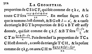
Here is an extract from the most helpful 1925 edition of David Eugene Smith and Marcia Latham[4], including a facsimile of the original 1637 edition of La Géométrie opposite their English translation. This is from Book I, where Descartes takes up Pappus's problem. Note the free use of letters and fraction bar on the second line:
\[ CF \hspace{8px} \text{sera} \hspace{8px} {{ezy + dek + dex} \over {zz}}. \]
Descartes often uses "sera" (will be) for equals, but also the odd symbol appearing on the last line, a backwards "is proportional to" sign (\( \propto \)) as we'd write it today. He was just about the first to use superscripts for exponentiation — \( z^3, z^4 \), and so on (Cajori, §297-298), but usually preferred \( zz \) to \( z^2 \). The plus and minus signs were mostly standardized by the 1630s, having first been introduced in print by Johannes Widmann (Bohemian, writing in German) in 1489 in a mercantile arithmetic. Notice Descartes' (even then) non-standard but recognizable versions - see Cajori, §200-213, for an exhaustive discussion of the diffusion of the plus and minus signs and their variations. The square root sign \( \sqrt{\cdot} \) also has a provenance preceding Descartes by a hundred years (Cajori, §327).
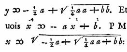
This extract from earlier in the work shows that Descartes' square roots are identical to ours:
\[ y = {- {1 \over 2}a + \sqrt{{1 \over 4} a^2 + b^2}}. \]
\[ x = \sqrt{- {1 \over 2}a + \sqrt{{1 \over 4} a^2 + b^2}}. \]
The equations are familiar and concern solving quadratic equations geometrically, an old subject going back to Euclid. Apart from \( aa \) for \( a^2 \) and the funky equals sign, Descartes' square root formulas could be found in any modern textbook. You can even see \( x^2 \) and \( b^2 \) slipping into the middle formula, as well as \( x^4 \).
The Pappus Problem
Pappus of Alexandria (~ 290-350 AD) was the last great mathematician of antiquity, known for his multi-volume Collection, an extensive compendium of then-known mathematics with commentary. Some otherwise lost work of his predecessors is known only through Pappus; he was much more than a simple conduit, being credited today as a precursor of projective geometry. Here is the Problem of Pappus at the center of Book I of La Géométrie:
Given four lines in the plane, consider points C making fixed angles when connected to those lines. Then the locus of all such points C such that \( {{CD \cdot CF} \over {CB \cdot CH}} \) equals a fixed constant is a conic section.
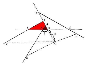
The diagram is straight from the 1925 Smith / Latham facsimile of the 1637 edition, other than the coloring and labeling \( x = AB \) and \( y = BC \) as Descartes explained. The four solid lines are the ones originally given — FS, and so on. The four dotted lines emanating from C make fixed angles with those four lines — ∠CFS is one of the given angles, for example.
Let's retrace Descartes. x and y will vary as C is repositioned; the objective is to express the lengths of the four line segments in terms of \( x = AB \) and \( y = BC \), then see what curve that determines. Line CB makes a fixed angle with line EG by the conditions of the problem, and also with lines DR and EG, since all those solid lines are fixed. Therefore the angles of ΔABR (the little triangle ▲ colored in dark red) are fixed as well, and by the Law of Sines, the ratio of sides is fixed too, say:
\[ {AB \over BR} = {z \over b}. \]
It's just the ratio that matters, not the values of b or z, though they will be used in what follows. Recasting:
\[ BR = {bx \over z}. \]
Therefore from the figure:
\[ CR = {BC + BR} = {y + {bx \over z}}, \]
where the plus sign would be a minus if R lied between C and B, and which it is doesn't affect the subsequent argument. In a similar way "the three angles of the triangle ΔDRC are known, and therefore the ratio between the sides CR and CD is determined." Descartes retains z from above and introduces a new constant c to express this ratio:
\[ {CR \over CD} = {z \over c}. \]
\[ \therefore CD = {{cy \over z} + {bcx \over z^2}}. \]
So we have \( CD \), one of the line segments to be measured, in terms of x, y, and constants. Now let \( k = AE \), a constant value determined by the original lines, so \( EB = {AE + EB} = {k + x} \), or maybe \( k - x \), it doesn't matter which (the former is used in what follows). All angles of ΔESB (colored in red ▲, both shades) are known, so the ratio of sides of that triangle is also known, say:
\[ {BE \over BS} = {z \over d}. \]
\[ \therefore BS = {{dk + dx} \over z} \hspace{10pt} \text{and} \hspace{10pt} CS ={{zy + dk + dx} \over z}. \]
Pappus Problem worked example from La Géométrie
From CS we can get CF, because ΔFSC has known angles and therefore its sides too are in a fixed ratio and:
\[ {CS \over CF} = {z \over e}. \]
\[ \therefore CF = {{ezy +dek + dex} \over z^2}. \]
Looking back at the statement of the theorem, we now have expressions for the numerator \(CD \cdot CF \). Continuing in this vein, constants l, f and g are introduced and \( CH \) is calculated:
\[ CH = {{gzy + fgl - fgx} \over z^2}. \]
We now have all four pieces determining the locus in the theorem's condition, recalling that \( y = BC \):
\[ {{CD \cdot CF} \over {CB \cdot CH}} = \text{a fixed constant}. \]
This all follows Descartes closely. He proceeds:
And thus you see that, no matter how many lines are given in position, the length of any such line through C making given angles with these lines can always be expressed by three terms, one of which consists of the unknown quantity y multiplied or divided by some known quantity; another consisting of the unknown quantity x multiplied or divided by some other known quantity; and a third consisting of a known quantity. ... You also see that in the product of any number of these lines the degree of any term containing x or y will not be greater than the number of lines (expressed by means of x and y whose product is found. Thus no term will be of degree higher than the second if two lines be multiplied together, nor of degree higher than the third, if there be three lines, and so on to infinity.
That's pretty clear. To continue spelling it out, I'll introduce Greek letters for the new constants (themselves expressions involving b, c, d, etc.):
\[ {{CD \cdot CF} \over {CB \cdot CH}} = {{{(\alpha x + \beta y)} \cdot {(\gamma x + \delta y + \epsilon)}} \over {y \cdot{(\zeta x + \eta y + \theta)}}} = \iota. \]
\[ \therefore {{(\alpha x + \beta y)} \cdot {(\gamma x + \delta y + \epsilon)}} = {\iota \cdot y \cdot {(\zeta x + \eta y + \theta)}}. \]
Multiplying out and collecting together the coefficients of the variables, denoted by capital Greek letters:
\[ {\Gamma x^2 + \Delta xy + \Theta y^2 + \Lambda x + \Upsilon y} = 0. \]
Click image for Pappus's original text.
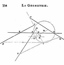
Now we're talking — that's a conic section! In Book II (pp 324-335), Descartes examines this equation in detail, considering how the outcome varies as the constants are juggled. He notes that the resultant locus can be a straight line, a circle, an ellipse, a parabola, or a hyperbola, depending how the constants are related to each other. He traces curves in a number of cases and calculates geometric properties like the center and latus rectum. He walks through a specific example leading to a circle. In Book II, he says this:
I could give here several other ways of tracing and and conceiving a series of curved lines, each curve more complex than any preceding one, but I think the best way to group together all such curves and then classify them in order, is by recognizing the fact that all points of those curves which we may call "geometric", that is, those which admit of precise and exact measurement, must bear a definite relation to all points of a straight line, and that this relation must be expressed by means of a single equation.
Smith and Latham note that this statement contains the fundamental concept of analytic geometry. Descartes' very next sentence states that if the equation contains the unknowns in only the first or second degree, then the curve it represents is a conic section.
The construction assumes that the original four lines intersect each other. It's fine if there are only three lines, then one of them is used twice and that product becomes a square. In Book II, Descartes considers the case where the original four lines are parallel, a different but also interesting problem. He considers cases where there are more than four lines, leading to higher level curves. Judith Grabiner follows him more closely in her excellent article "Descartes and Problem Solving"[5], and includes great references as well.
Fermat and Analytic Geometry
In 1636, Pierre de Fermat wrote a twenty-page work, Ad Locos Planos et Solidos Isagoge ("Introduction to Plane and Solid Loci"), establishing him as the co-inventor of analytic geometry. The Isagoge contains the following, called by Boyer "one of the most significant statements in the history of mathematics" ( p 75):
Whenever in a final equation the two unknown quantities are found, we have a locus, the extremity of one of these describing a line, straight or curved.
According to Boyer, Fermat was more methodical than Descartes in developing equations for the straight line and conic sections and sometimes started with equations rather than always deriving them, a huge step that he was first to take. Fermat used the notation of Viète, representing, for example, the Witch of Agnesi like this (Boyer, p 81):
\[ Bc. \hspace{5px} \text{aequalis} \hspace{5px} Aq. \hspace{5px} \text{in} \hspace{5px} E + Bq. \hspace{5px} \text{in} \hspace{5px} E. \]
Capital letters represent values, with vowels for unknowns and consonants for constants. The little c on the left means to cube the constant B. Similarly Aq. means A². "In" is used for multiplication, perhaps a remnant of geometric thinking, where a product of two lines is thought of as the area of the rectangle they make. So it would be this in our notation:
\[ b^3 = {x^2 y + b^2 y}, \]
and that's how Descartes would have written it. It was Descartes' notation that took the world by storm and was adopted almost instantly. Although known by some French mathematicians, Fermat's work wasn't even published until after his death in 1679. Compare to La Géométrie, first published in 1637 to some fanfare, then systematically consolidated and extended by many mathematicians as the 17th century progressed.
Dissemination through van Schooten Editions
Frans van Schooten (1615-1660).
Frans van Schooten (Dutch, 1615-1660) met Descartes as a boy in Leiden (his father was a mathematician). He was a bit of an artist and illustrated La Géométrie when first published in 1637. Developing as a mathematician himself and in continuing contact with Descartes, he recognized both the importance of Descartes' work and its opacity. Descartes was recognized as a thinker, but his Géométrie, published as an appendix in a longer work explicitly to make a philosophical point, badly needed to be organized and expounded if it were to extend its reach. That organizer was van Schooten, < href="http://www.maa.org/publications/periodicals/convergence/the-geometry-of-rene-descartes">who published editions of La Géométrie in 1649 and 1659-61 and gets some posthumous credit for the 1681 edition as well. van Schooten translated Descartes's French into Latin, adding his own commentary and that of others, including de Beaune, Hudde, Heuraet, and de Witt, eventually to the extent that the added material dwarfed the original. Descartes' mathematical reputation was cemented by the 1659-1661 edition, an epochal work < href="http://en.wikipedia.org/wiki/Frans_van_Schooten">studied carefully by the new generation of scholars who built calculus on top of analytic geometry.
van Schooten's commentary included chapter-and-verse exegesis in places, supplementary discussion and exercises in others. The long commentary CCC in the 1659-61 edition took up the foundations of Apollonius's old work on conics, which played an important role in La Géométrie. In Book II, Descartes developed a theory of normals to curves involving circles - it was cumbersome and soon superseded, but fruitful all the same. He sets out to apply the method to an ellipse and includes a diagram:
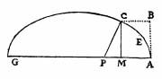
For example, if CE is an ellipse, MA the segment of its axis of which CM is an ordinate, r its latus rectum, and q its transverse axis, then by Theorem 13, Book I, of Apollonius, we have \( x^2 = {ry - {r \over q} y^2} \). Eliminating \( x^2 \) the resulting equation is \( \cdots \).
Stop right there! That's the equation of an ellipse as we might write it today, considering that r and q are positive. There is a theorem that the latus rectum \( = r = {2b^2 \over a} \) and here \( q = 2a \), where a and b are the lengths of the ellipse's two axes, as usual — with these two substitutions, Descartes' equation can be beaten into the canonical equation of an ellipse in short order. van Schooten develops that passage in commentary L, including an enhanced diagram (as good a translation as I can produce):
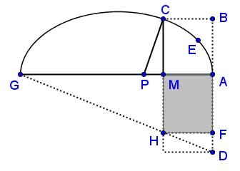
For let AD = r be the length of the latus rectum, dropped down perpendicular to AG. Because triangles GAD and HFD are similar, and GA and AD equal q and r respectively, and HF = MA = y, we have:
\[ {q \over r} = {GA \over AD} = {HF \over FD} = {MA \over FD} = {y \over FD}, \]
and so FD = \( {ry \over q} \). If we multiply that by y = HF, then rectangle HFD has area \( ry^2 \over q \). And then by Apollonius's Conics, Book I, Proposition 13, the area of rectangle MAD minus the area of rectangle HFD equals the area of the square on CM; and indeed the area of rectangle MAD is ry, so the area of rectangle MAF = \( {ry - {ry^2 \over q}} \). And therefore the equation is: \( x^2 = {ry - {r \over q} y^2} \cdots \)
A number of points are in order. The diagram is reproduced straight from van Schooten, other than the coloring, and probably came from his hand. Like van Schooten says, Book I, Proposition 13 of < href="https://archive.org/stream/treatiseonconics00apolrich#page/10/mode/2up">Apollonius's Conics equates the area of the gray rectangle with the area of the square on CM, where AD is the length of the latus rectum. The theorem is true as point M runs along axis AG, that's the point! This is a key theorem early in the work, where Apollonius pulls the ellipse down from the three dimensional cone and derives a relation in the plane characterizing the ellipse. Apollonius named the ellipse from this property, that the gray rectangle is less than the larger rectangle MAD on the latus rectum, the Greek root "ἔλλειψις / elleipsis" meaning "falling short" or "having a deficit" ("ellipsis" in English has the same root \( \cdots \)).
Note also that x and y are reversed compared to all subsequent usage, with y marking off along the horizontal axis, x along the vertical. We have caught an early moment when Cartesian analytic geometry is already committed to the letters x and y as unknowns, but not to which dimension each letter referred. Also when it is perfectly willing to use rectangular coordinates to help solve a problem.
Geometric Constructibility
Ancient Greek geometers were obsessed with straightedge and compass constructions to the point of retarding the subject, a preoccupation carried over into the early modern period and the subject of extended commentary by Felix Klein as late as 1894. Descartes was not immune from this heritage, but proposed that the instrument set be expanded. In Book II, for example, he specifies a physical instrument producing a hyperbola (see Smith and Latham edition, p 50-55). He granted that such curves were a more complex species, as the ancients held ("solid" rather than the "plane" curves produced by straightedge and compass), but admitted them to polite company; indeed Books I and II are largely taken up with such "solid" curves.
He entertained a third species of still more complex curves, the "linear" ones resulting from cubic and higher order equations (see his account of the three types at the start of Book II). He would try to solve "linear" problems by intersecting conics. Book III takes up finding roots of higher order polynomial equations. Of course the cubic and quartic equations had been solved by Tartaglia and Cardan, but Descartes was willing to go higher - his celebrated rule of signs for the roots of polynomial equations is found here. Boyer calls Book III "an elementary course in the theory of equations, written in a language and notation almost identical with that in modern textbooks" (p 96).
Instruments based on physical properties of the conic sections go back to late antiquity, especially Anthemius of Tralles (Byzantine, ~ 474-534), who considered many such contraptions and was aware of the string construction of the ellipse and the light-focusing property of the parabola. The fixation on physical constructibility did have a point, namely, to show that the modeled curve actually exists. It would be well-behaved as well, no chance of a Weierstrass monster. The insistence on constructibility might have held up progress, but it also guarded against premature consideration of pathological curves.
Jan De Witt's Elementa Curvarum Linearum
Jan De Witt (1625-1672) was a Dutch statesman who became the Grand Pensionary of Holland, an office which, according to Albert Grootendorst, was equivalent to today's Prime Minister plus Minister for Foreign Affairs. In his early twenties, de Witt composed the core of Elementa Curvarum Linearum, published as an appendix of the 1659-61 edition of La Géométrie. Boyer says the second book of Elementa "is so systematic a treatment of analytic geometry that it has been described as the first textbook on the subject" (p 114), a sentiment echoed by Grootendorst in his English translation Jan de Witt's Elementa Curvarum Linearum, Liber Primus[6].
Drag red point along ellipse
Elementa has two books. The first was in the ancient synthetic tradition, but interesting as an example of that and Cartesian in its kinematic approach to defining the conic sections. The ellipse, for example, is defined as the locus of a point moving at the end of a rod with two fixed points moving along two fixed axes. Drag the red point along the ellipse in this diagram to get the idea: the two black points are in fixed positions on the rod, but the rod itself moves so that the black points slide along the x and y axis respectively. This works fine if the axes are not at right angles and it's an old idea, the trammel of Archimedes, and not hard to prove it leads to an ellipse with major semi-axis the length of the rod and minor semi-axis the length of the segment of the rod closer to the ellipse (the longer one in the diagram). Drag the red point so the rod is horizontal to see it coincide with the major semi-axis, and similarly when the rod is vertical.
In short order, de Witt proves the chord theorem mentioned above as being characteristic of ellipses — his Book I, Theorem XII, couched though it is in his own terminology of directrix and secant and the rest (Corollary 1 is more clear). Then he brings it home (Grootendorst translation, Liber Primus, p 146-147 — note the highlighted passages correspond):
Atque ita liquet, praedictam curvam eam ipsam esse, quae Veteribus Ellipsis dicta fuit, directricem vero ac secantem eas ipsas, quas conjugatas diametros, aut, si angulus rectus fuerit, conjugatos axes vocarunt.
Thus it is clear that the said curve is the same as the curve that was called "ellipse" by the Ancients and that the directrix and secant are the same as what they called conjugate diameters or — if the angle should be a right angle — conjugate axes.
In the second book[7], de Witt systematically develops the equations for the conic sections, including the straight line. Fermat got a start on this with his short Isagoge, archaic though the notation. John Wallis in England was doing a good job in this vein as well, but de Witt was the first follower of Descartes to develop this approach systematically and lay down a series of equations. For example, this diagram accompanies Theorem XIV in Book II, where de Witt generates the equation of the ellipse (except for the dashed line and point S, which I added). Van Schooten likely drew the published diagram, where GF is the length of the latus rectum (the ellipse's "parameter" in de Witt's terminology). Point A is the origin, x an unknown progressing to the right, and y up, just as we would do. That de Witt or van Schooten illustrated the theorem with perpendicular axes is itself striking, because it holds generally for oblique conjugate axes, or "conjugate" diameters" as they were called by the ancients. de Witt's original Latin is on the left, Grootendorst's English translation — for the most part — on the right (Liber Secundus, p 132):
Elementa Curvarum Linearum, Book II, Chapter III, Theorem XIV
Si aequatio sit \( {l yy \over g} = {ff - xx} \), erit Locus quaesitus Ellipsis.
Hinc ad praedicti Loci determinationem esto in apposita figura ipsius x initium immutabile A punctum, atque eadem x se per lineam AE ab A versus E indeterminate extendere intelligatur, sitque angulus, quem y & x comprehendunt, aequalis angulo AGF. Porro cum sit ut l ad g, ita ff - xx ad yy: facile apparet, si tam AG quam AC sumantur aequales f cognitae; fiatque ut l ad g, ita CG ad GF, ac centro A, transversa diametro CG, & parametro GF Ellipsis descibatur GDC, eandam curvam GDC fore Locum quesitum. \( \cdots \)
If the equation is \( {l y^2 \over g} = {f^2 - x^2} \), then the required locus will be an ellipse.
Hence, to determine the aforementioned locus, in the figure here let point A be the immutable initial point of x, and let us suppose that this x extends indeterminately along line AE from A toward E, and let the angle enclosed by y and x be equal to the angle AGF. Then the following is easy to see because f² - x² is to y² as l is to g: if both AG and AC are supposed to be equal to the known f, and if we make CG to GF as l is to g, and if we describe the ellipse GDC with A as its center, CG its transverse diameter, and GF its parameter, then this curve GDC will be the required locus. \( \cdots \)
To parse this, notice that A is the origin, the immutable initial point and that x extends away from it indeterminately along a straight line — along a horizontal axis and to the right in the diagram. The next paragraph of the proof (not shown), identifies y with ED, which is oriented towards transverse diameter CG (the major axis of the ellipse) in the direction of its conjugate diameter — perpendicular in the diagram but not necessarily so, considering that the enclosed angle can be oblique. GF rises from the major axis in a direction conjugate to it (90° here) and has the length of the ellipse's latus rectum — de Witt calls GF the "parameter" of the ellipse. l, g and f are constants (known values), in keeping with Descartes' naming convention. De Witt says \( {{(f^2 - x^2)} / y^2} = {l / g} \), where \( f = AG = AC \) is the semi-major axis.
De Witt brings the latus rectum GF into it, for which the old boys had an inordinate fondness, but the result follows directly from his own Book I, Theorem XII, mentioned just above:
\[ {y^2 \over {f^2 - x^2}} = {y^2 \over {{(f - x)} \cdot {(f + x)}}} = {DE^2 \over {CE \cdot EG}} = {AS^2 \over AG^2} = {g \over l}. \]
Keep in mind that we are given positive constants l and g — it turns out that they are the squares of the semi-minor and semi-major axes of the ellipse, respectively (or at least are in the same ratio); also positive constant f, which turns out to be the semi-major axis. In addressing this equation just past the quote above, de Witt speaks of "the rectangle CEG", employing the old geometric language for CE · EG.
Change of Axes in Elementa
Shortly after the discussion of Theorem XIV, de Witt shows how to reduce an equation to his canonical form. The section is titled Exemplum reductionis aequationem ad formulam Theorematis XIV (Example of the reduction of equations to the form of Theorem XIV) and can be found at page 296 of the 1659-61 edition. His general equation is:
\[ {y^2 + {2bxy \over a} - 2cy} = {-x^2 + dx + k^2}. \hspace{40px} (0) \]
In one page, he builds a transform converting \( (x, y) \) coordinates to \( (v, z) \) coordinates such that the equation in \( v \) and \( z \) satisfies the canonical form of Theorem XIV. You can follow it with a little Latin, or see Grootendorst's translation (better yet, his summary on page 39 of Liber Secundus):
 \[ {v = x - h}, \hspace{10pt} {z = y - c + {bx \over a}}, \hspace{40px} (1) \]
where \( h \) is an expression containing \( a, b, c, \) and \( d \). Let's do a worked example with:
\[ a = 2, \hspace{6pt} b = 1, \hspace{6pt} c = 2, \hspace{6pt} d = 3, \hspace{6pt} k = 1. \]
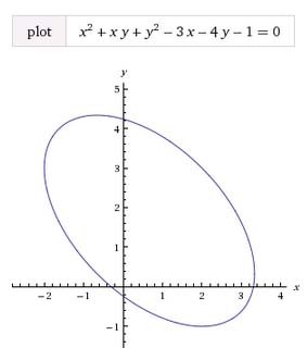
The task (after rearrangement) is to reduce this equation to canonical form:
\[ {x^2 + xy + y^2 - 3x - 4y - 1} = 0. \hspace{40px} (2) \]
De Witt develops expressions for \( l/g \) and \( f^2 \) in terms of the coefficients of (2) which, in this example, reduce to:
\[ {l \over g} = {4 \over 3}, \hspace{20pt} f^2 = {64 \over 9}, \]
so the reduced equation is:
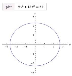
\[ \begin{equation}{{{lzz \over g} = {ff - vv}} \hspace{8pt} \equiv \hspace{8pt} {{4z^2 \over 3} = {{64 \over 9} - v^2}} \hspace{8pt} \equiv \hspace{8pt} {{9v^2 + 12z^2 - 64} = 0}.} \tag{3} \end{equation} \]
This process is not equivalent to the modern one involving only a rotation and translation, which reorients the ellipse but preserves its shape. De Witt's transform rotates and translates, but also dilates the original coordinates to produce the new ones. (0) is close to the general equation for a conic and includes all ellipses when \( a^2 > b^2 \). He has extended geometric discussion about this reduction, but his lasting contribution is to posit canonical equations for the straight line, ellipse, parabola, and hyperbola and prove that all second degree equations can be reduced to one of them:
Regula Universalis (General Rule) in Elementa
Regula universalis, modusque reducendi omnes aequationes, quae ex convenienti operatione existunt, cum Locus vel Hyperbola est, vel Ellipsis, vel Circuli circumferentia, ad aliquem quatuor casuum praecedentium, totidem Theorematibus jam explicatorum.
Universal rule and method of reducing all equations which arise from suitable operations (whether the locus is a hyperbola, an ellipse, or the the circumference of a circle) to one of the four preceding cases, each with its own theorem, as already explained.
Descartes' Legacy
René Descartes was one of the more amazing thinkers who ever lived, whose very errors were fruitful (his vortex theory in astronomy, for example). Bertrand Russell said that Descartes is usually, and rightly, considered the founder of modern philosophy, foremost in style as well as thought. In geometry as in philosophy, he bridged old and new. Analytic geometry would have developed along its course had Descartes never touched it — witness his contemporaries Fermat and especially John Wallis in England, decidedly, even vociferously, not of the Cartesian tradition (he accused the Cartesians of stealing from him).
All the same, Descartes and his acolytes quickened the pace by establishing new universally adopted notations — \( a, b, c, \cdots \) and \( x, y, z, \cdots \) for variables and superscripts for powers. According to Florian Cajori, even the backwards \( \propto \) almost carried the day as a sign of equality (all the typesetters had to do was rotate their taurus zodiac sign counter-clockwise by 90°). It is hard to overestimate the power of mathematical notation as a spur to productivity. Here we have perfectly sound conventions that quickly became dominant, so mathematicians could read each other easily. Read Descartes, whose notation we use today, side-by-side with his contemporary Fermat, who arguably had a better, certainly a more systematic, sense of analytic geometry. Descartes is clear almost 400 years later, Fermat virtually unintelligible — it is a different language and not talking about the Latin, which is easy compared to his mathematical notation.
Descartes' golden touch brought the new subject to life in a momentous way one day in 1637. Descartes' geometry was lucky to have been embraced by Frans van Schooten, by all accounts a superior editor and illustrator, an industrious and generous organizer and friend to a circle of talented young Dutch mathematicians. The 1659-61 edition became a textbook for leading researchers, including Leibnitz and Newton, the foundation on which calculus was erected. Descartes' genius was understood and his work forwarded by this talented group of workers for fifty years until it became mainstream, that is the story of La Géométrie and its impact.
Mike Bertrand
October 13, 2014
^ 1. History of Analytic Geometry, by Carl B. Boyer, Scripta Mathematica (1956). In truth: p 27.
^ 2. A Concise History of Mathematics (4th Revised Edition), by Dirk J. Struik, Dover (1st ed. 1948, 4th ed. 1987), ISBN 978-0-486-60255-4.
^ 3. A History of Mathematical Notations, Vol I, by Florian Cajori. The Open Court Company (1928).
^ 4. The Geometry of René Descartes, David Eugene Smith and Marcia Latham, translators, The Open Court Publishing Company (1925).
^ 5. "Descartes and Problem Solving", by Judith Grabiner (Mathematics Magazine, Vol 68, No 2 — April 1995).
^ 6. Jan de Witt's Elementa Curvarum Linearum, Liber Primus by Albert W. Grootendorst, Springer (2000), ISBN 0-387-98748-7. equivalent to today's Prime Minister: p 4.
^ 7. Jan de Witt's Elementa Curvarum Linearum, Liber Secundus by Albert W. Grootendorst, et al., Springer (2012), ISBN 978-0-85729-141-7.